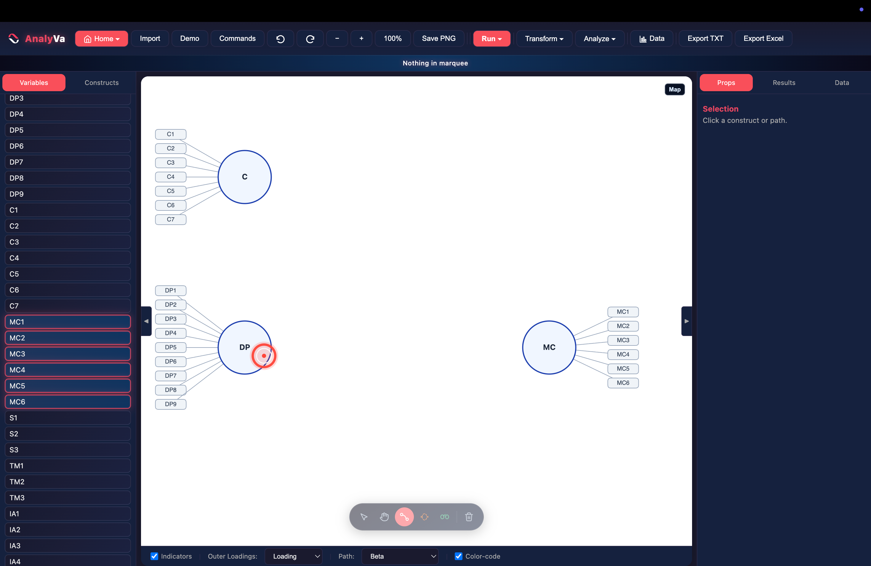
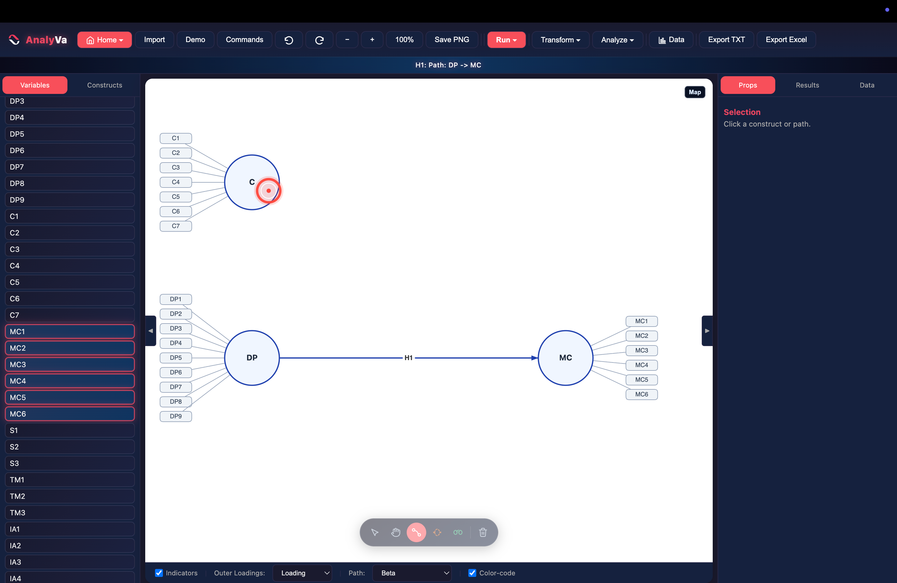
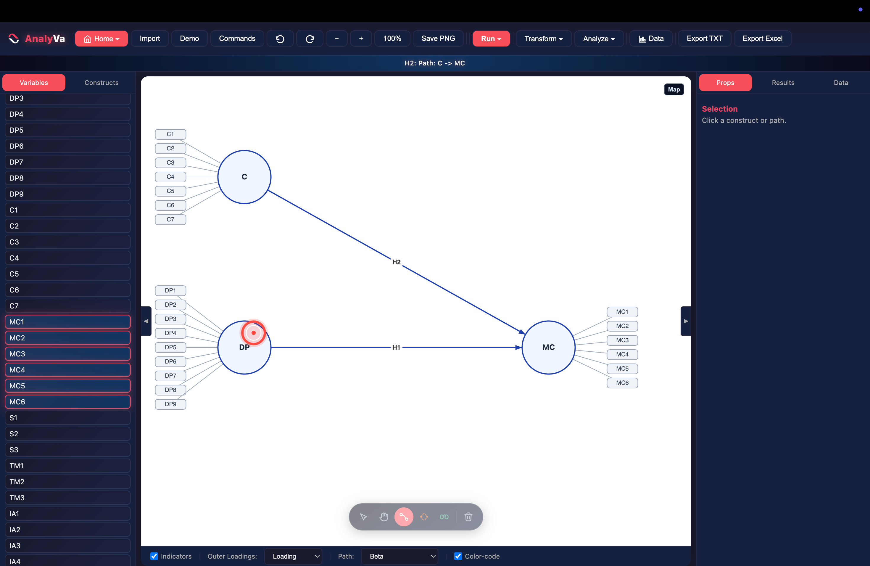
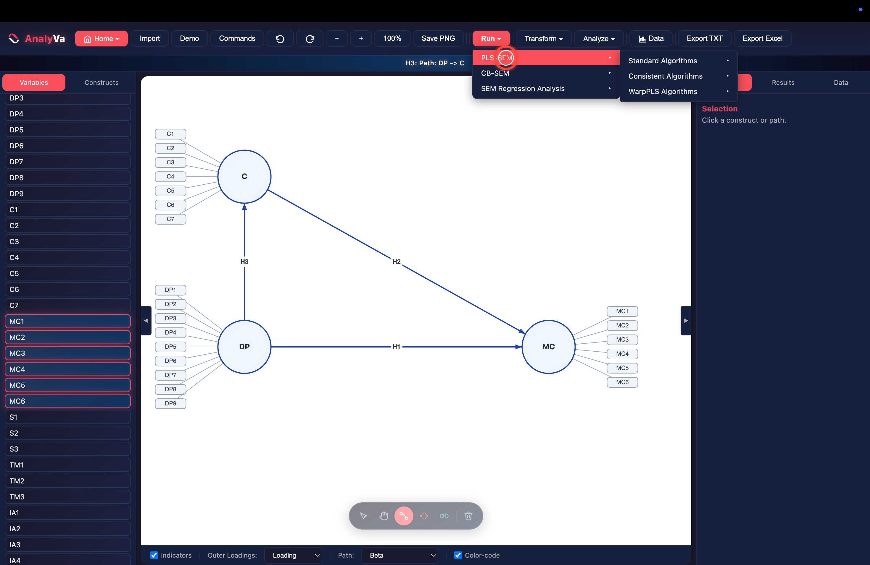
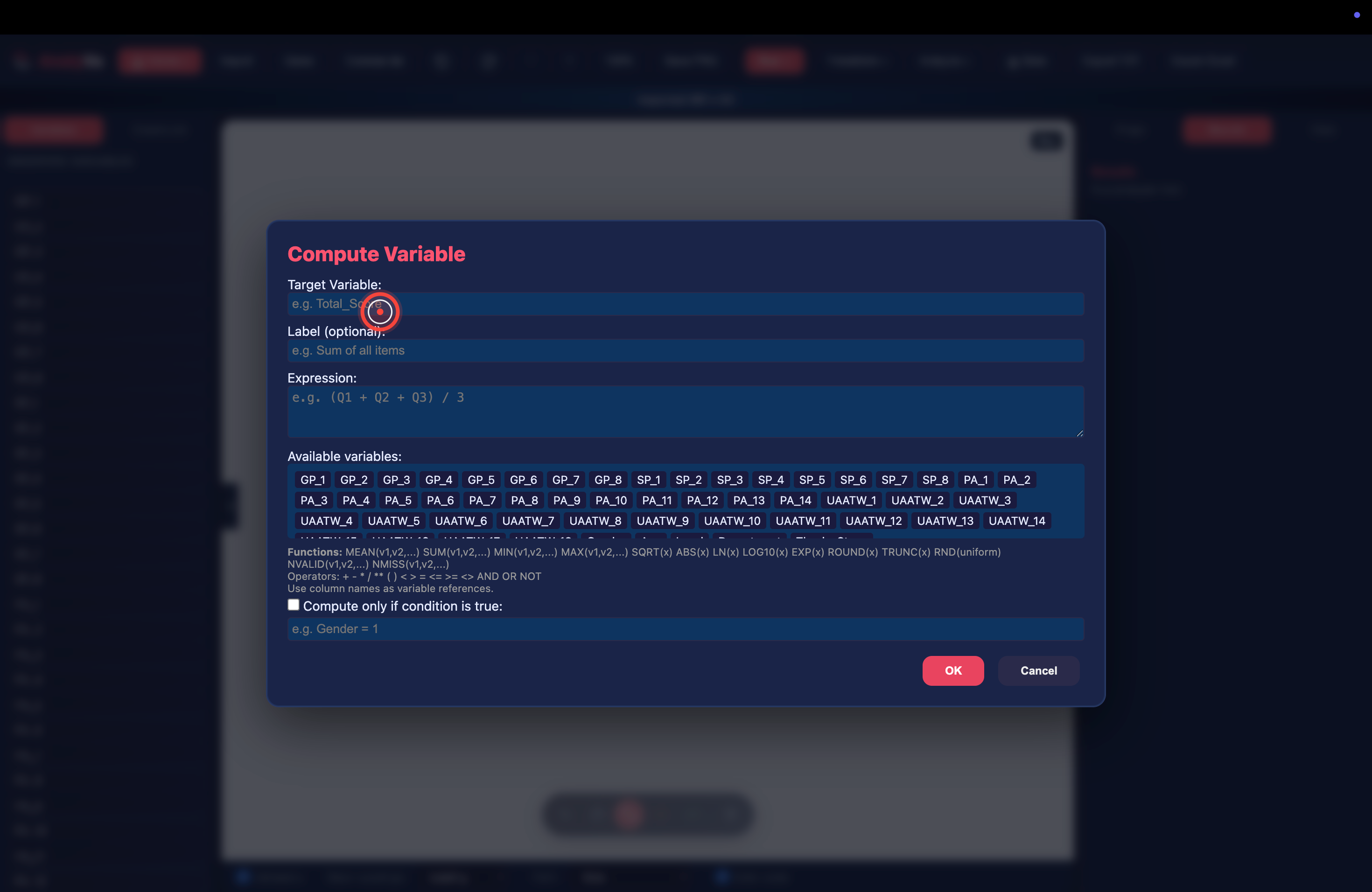
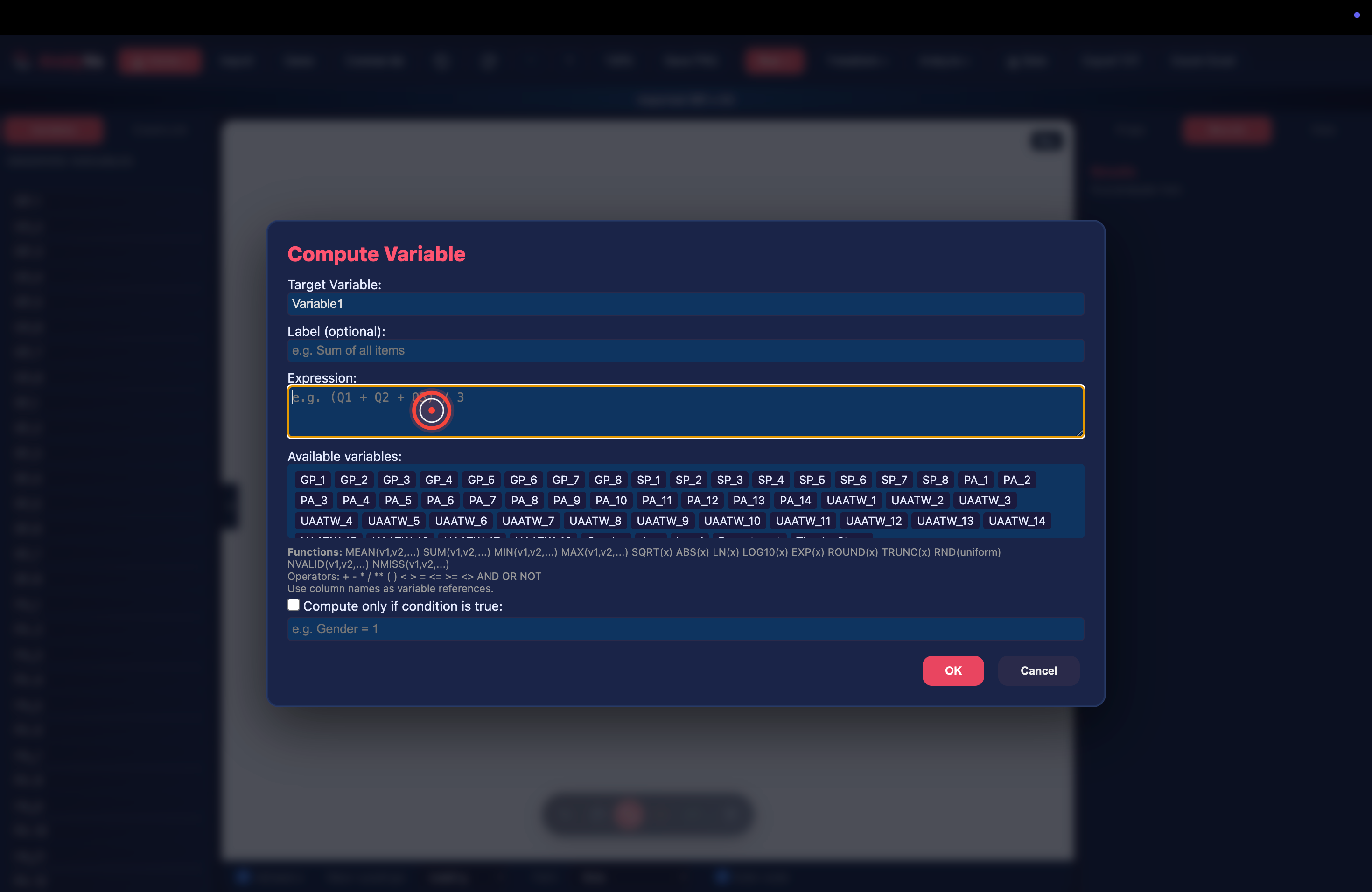
<?xml version="1.0" encoding="utf-8"?><feed xmlns="http://www.w3.org/2005/Atom" ><generator uri="https://jekyllrb.com/" version="3.10.0">Jekyll</generator><link href="https://analyva.com/feed.xml" rel="self" type="application/atom+xml" /><link href="https://analyva.com/" rel="alternate" type="text/html" /><updated>2026-09-03T10:13:20+00:00</updated><id>https://analyva.com/feed.xml</id><title type="html">AnalyVa</title><subtitle>AnalyVa combines PLS-SEM, CB-SEM, SPSS-like statistics, and NVivo-like textual analysis in one affordable desktop application. Benchmarked against R 4.4.0 and SmartPLS 4.</subtitle><author><name>Abdelouahd Bouzar</name><email>support@analyva.com</email></author><entry><title type="html">Moderation Analysis in PLS-SEM: Adding an Interaction Construct in AnalyVa</title><link href="https://analyva.com/blog/moderation-analysis-in-pls-sem/" rel="alternate" type="text/html" title="Moderation Analysis in PLS-SEM: Adding an Interaction Construct in AnalyVa" /><published>2026-08-08T00:00:00+00:00</published><updated>2026-08-08T00:00:00+00:00</updated><id>https://analyva.com/blog/moderation-analysis-in-pls-sem</id><content type="html" xml:base="https://analyva.com/blog/moderation-analysis-in-pls-sem/"><![CDATA[<p>Moderation is the PLS-SEM technique that gets misread most often: a
non-significant interaction term doesn’t mean the moderator doesn’t
matter, and a significant one doesn’t automatically mean it’s large.
This post picks up the four-construct model from the indicator-cleaning
walkthrough, adds a moderator, and runs it through AnalyVa’s full
significance pipeline — Beta, p-value, and significance-star display —
so the difference between “detected” and “meaningful” stays visible the
whole way through.</p>
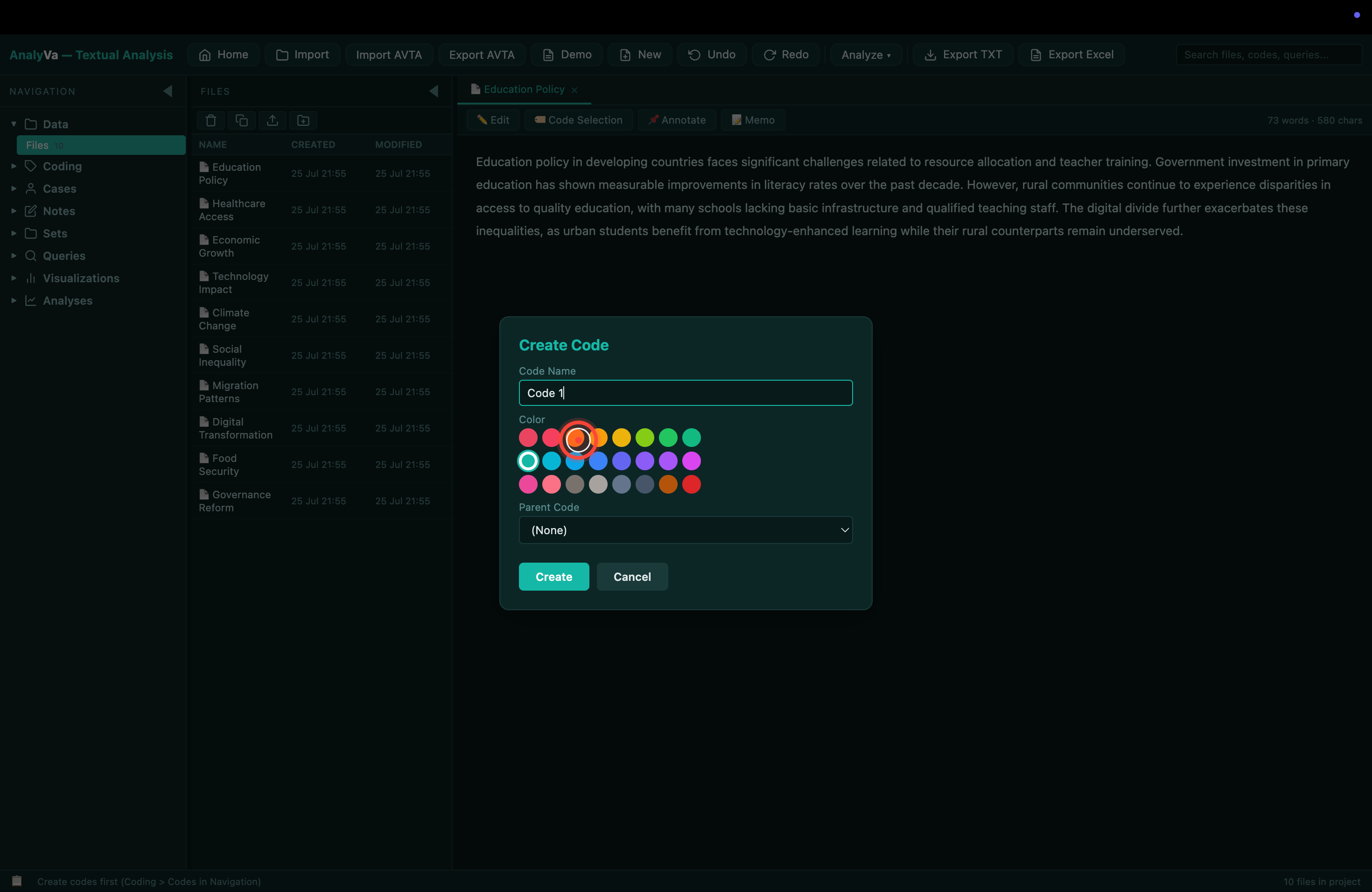
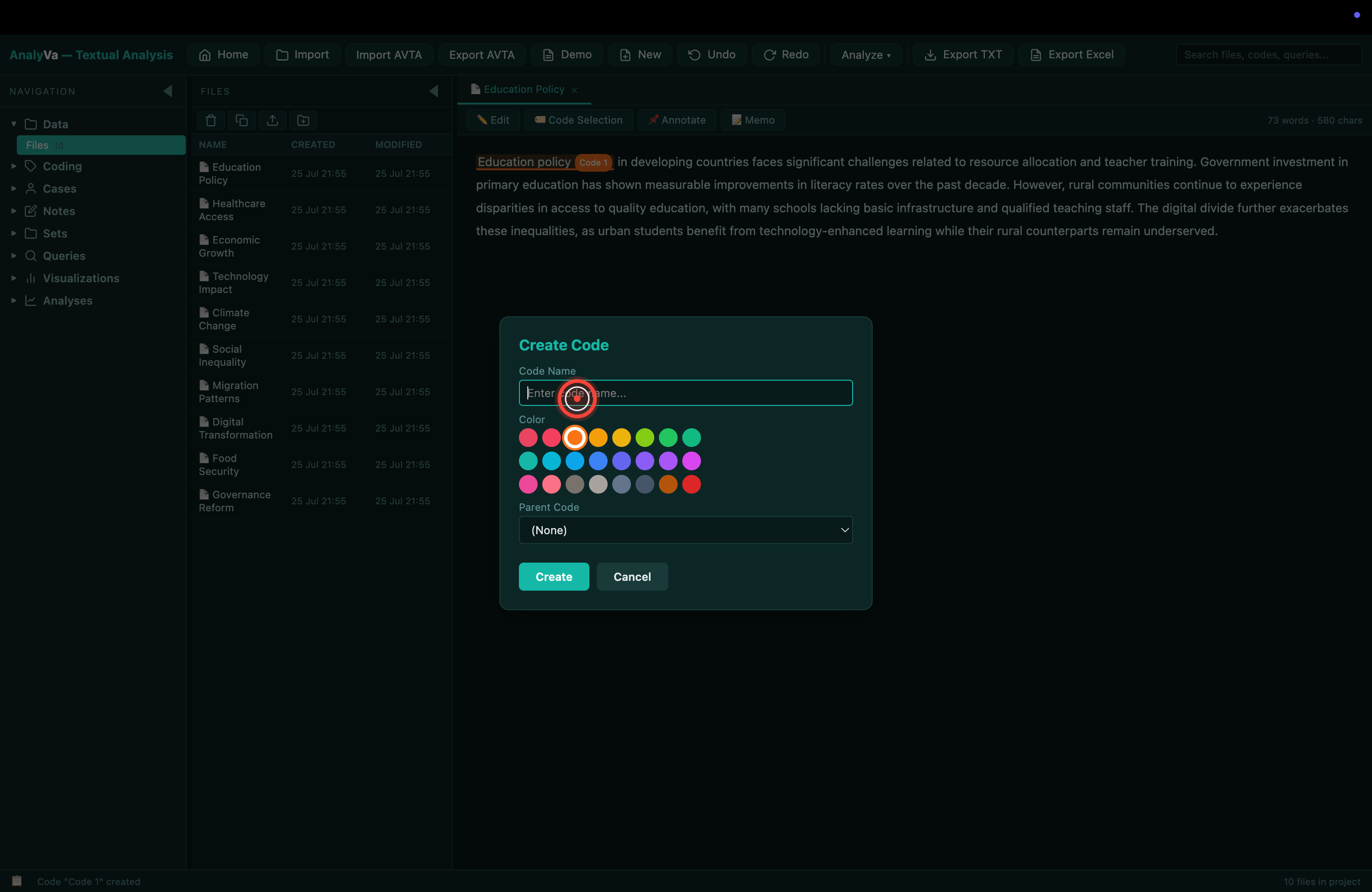
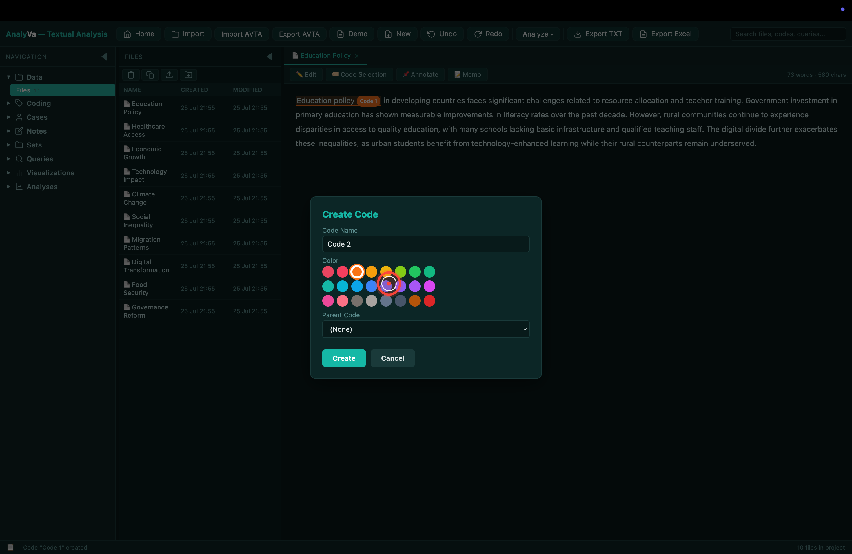
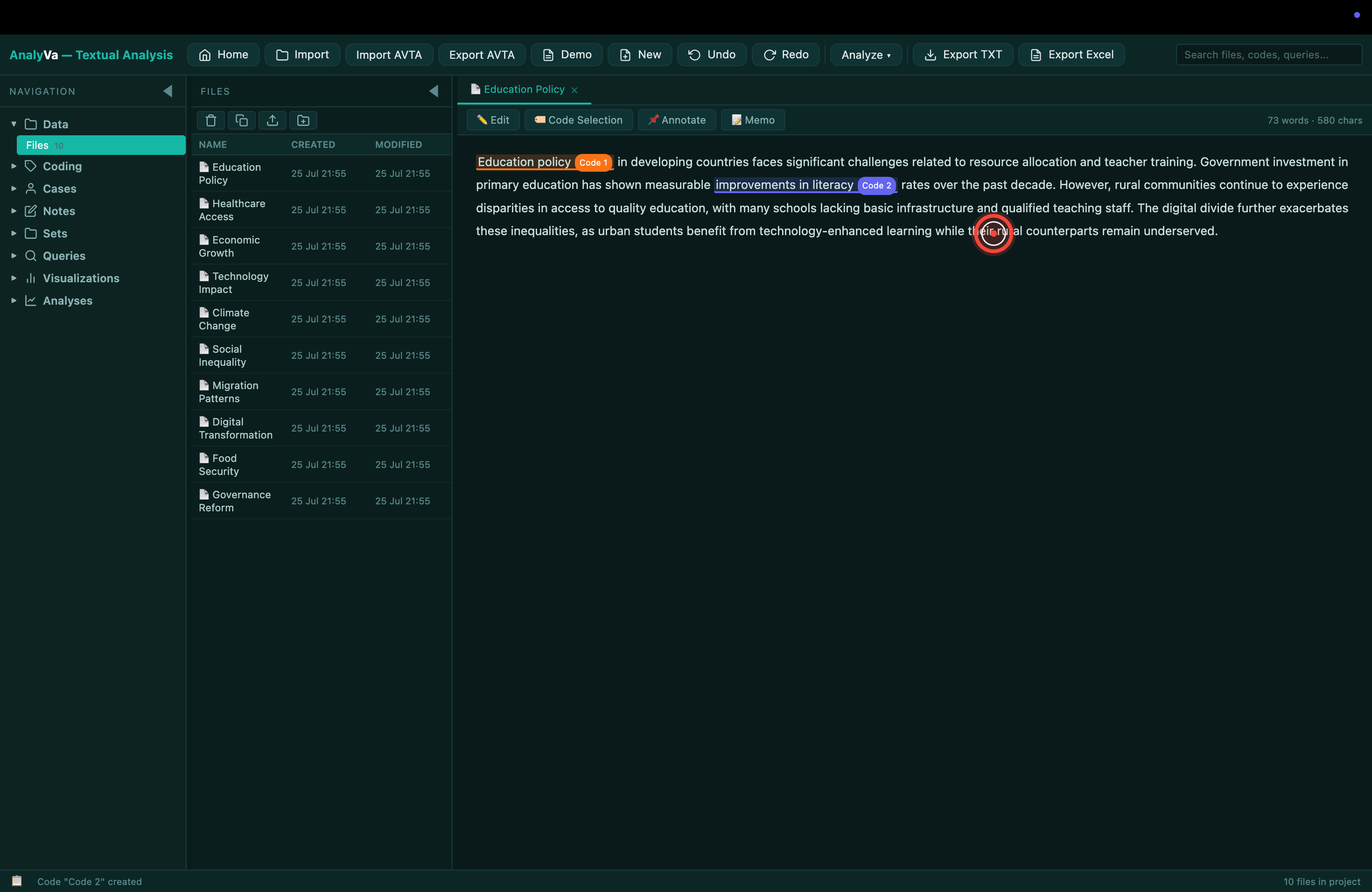
<h2 id="adding-the-moderator-construct">Adding the moderator construct</h2>
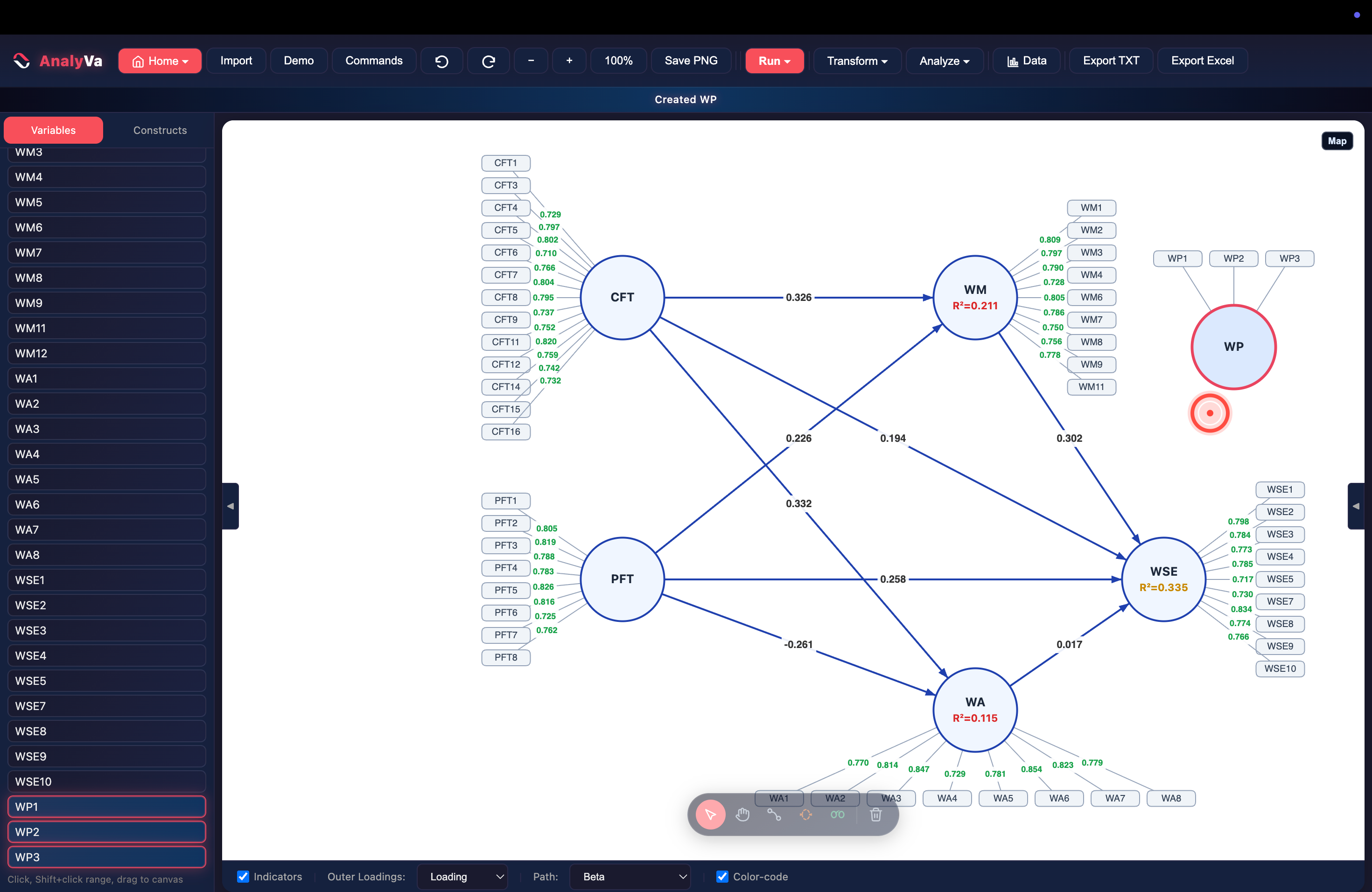
<p><strong>Step 1 — Build the WP construct from its indicators.</strong>
Select <code class="language-plaintext highlighter-rouge">WP1</code>–<code class="language-plaintext highlighter-rouge">WP3</code> in the sidebar the same way any other construct is
built (click, shift-click, drag to canvas). AnalyVa confirms with
<em>“Created WP”</em> and places it as a standalone construct, not yet
connected to anything.</p>

<p><img src="/blog/images/analyva-moderation-01.png" alt="WP construct created from WP1, WP2, WP3, sitting unconnected on the canvas" /></p>

<h2 id="drawing-the-interaction-paths">Drawing the interaction paths</h2>

<p>A moderator needs one interaction path per relationship it’s
hypothesized to moderate. This model tests four: does WP change the
strength of WM → WSE, WA → WSE, PFT → WSE, or CFT → WM?</p>

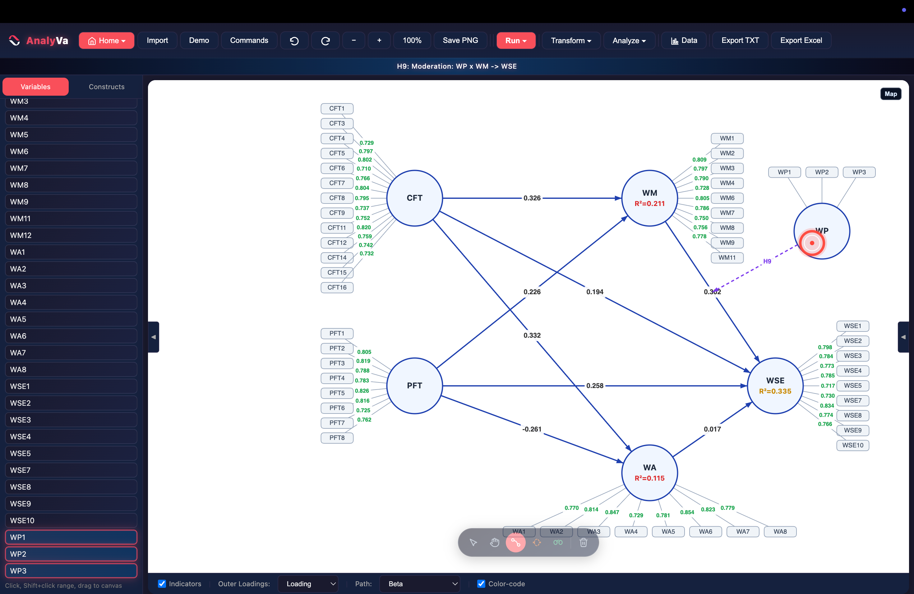
<p><strong>Step 2 — H9: WP × WM → WSE.</strong>
With the Path tool active, click WP, then click WSE. AnalyVa draws the
interaction as a dashed purple line — visually distinct from the solid
blue structural paths — and labels it automatically.</p>

<p><img src="/blog/images/analyva-moderation-02.png" alt="H9 interaction path drawn from WP to WSE, dashed purple" /></p>

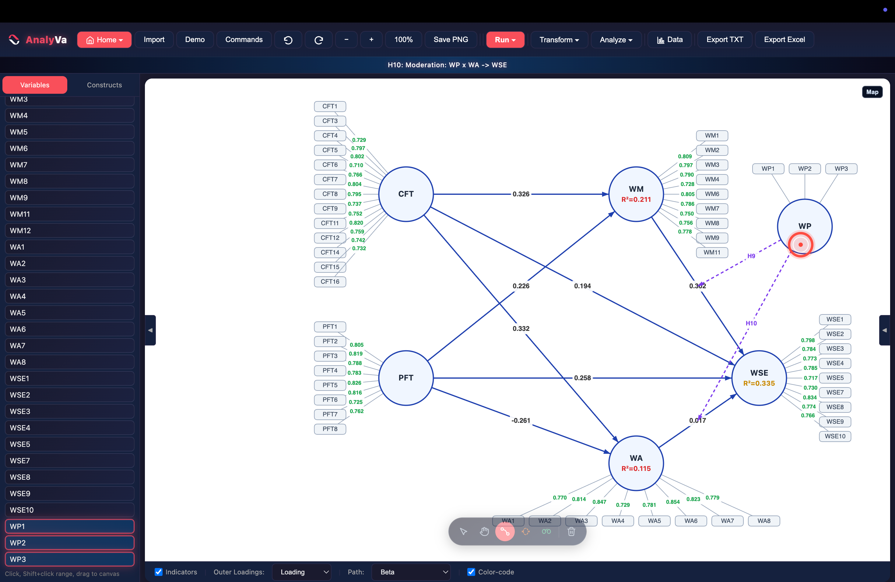
<p><strong>Step 3 — H10: WP × WA → WSE.</strong>
Same click-click pattern for the second interaction term.</p>

<p><img src="/blog/images/analyva-moderation-03.png" alt="H10 interaction path added, two dashed purple lines now visible" /></p>

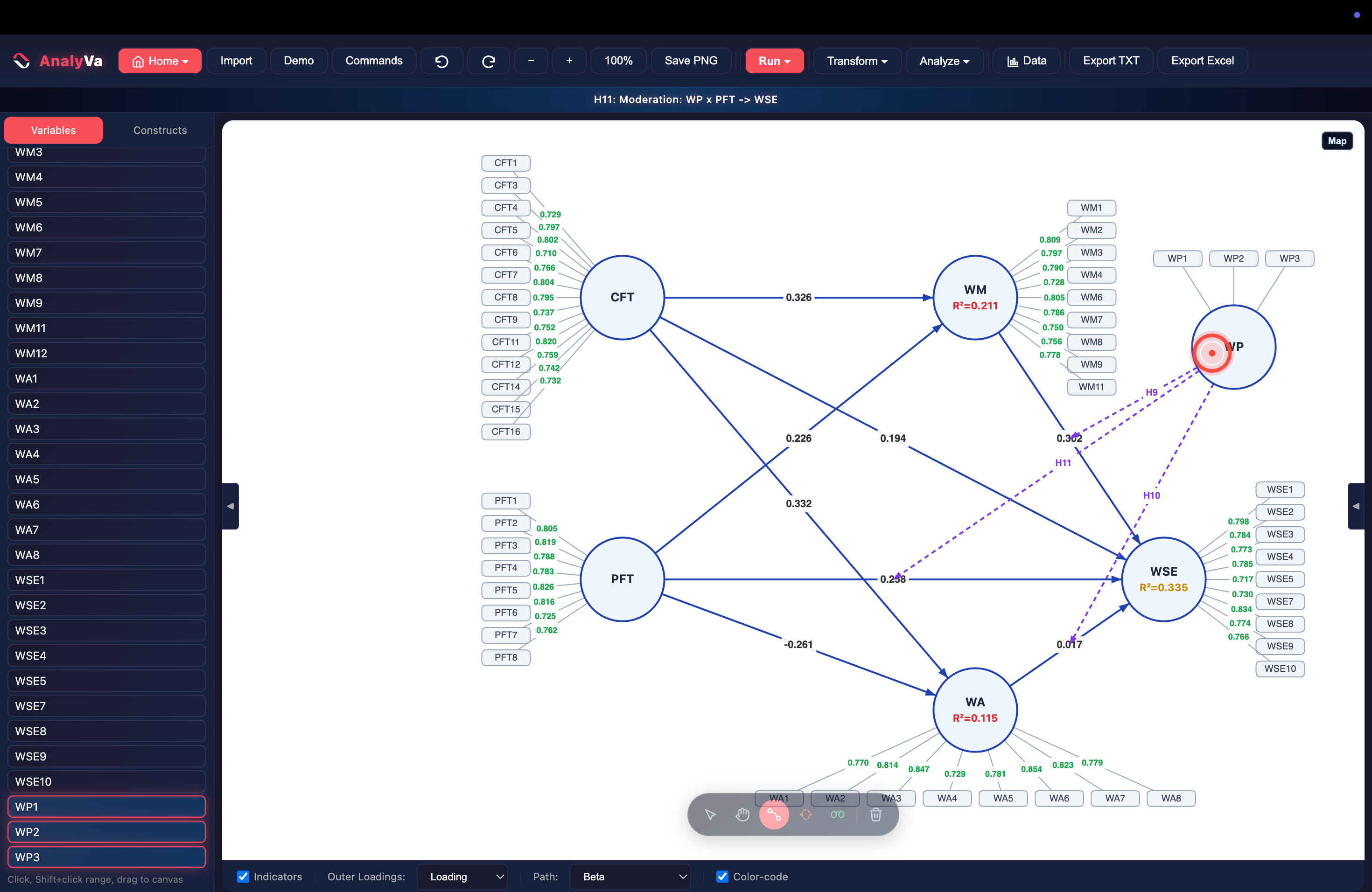
<p><strong>Step 4 — H11: WP × PFT → WSE.</strong>
A third interaction term, same pattern.</p>

<p><img src="/blog/images/analyva-moderation-04.png" alt="H11 interaction path added, three dashed purple lines converging on WSE" /></p>

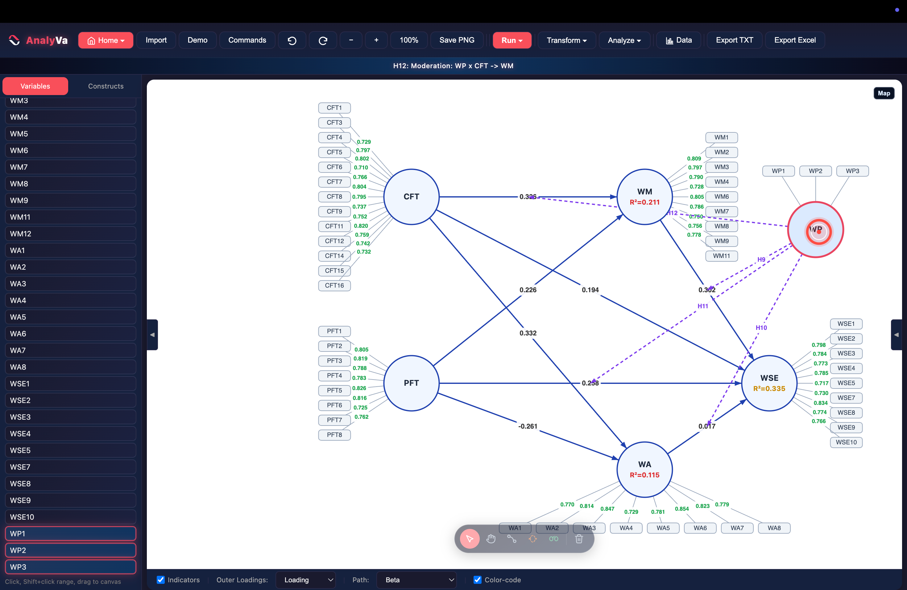
<p><strong>Step 5 — H12: WP × CFT → WM.</strong>
The fourth interaction targets WM instead of WSE — the moderator
doesn’t have to point at the same endogenous construct every time.</p>

<p><img src="/blog/images/analyva-moderation-05.png" alt="H12 interaction path added, all four moderation paths visible" /></p>

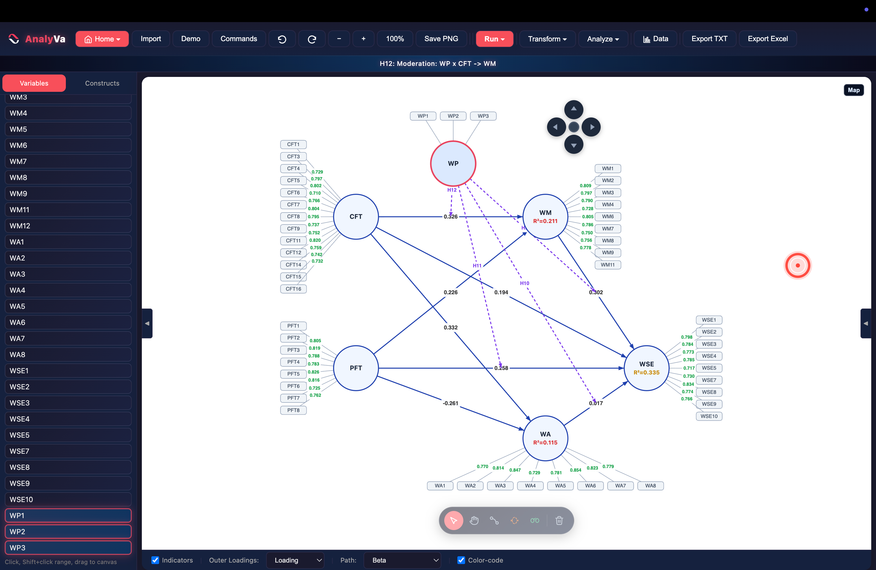
<p><strong>Step 6 — Reposition WP for a readable diagram.</strong>
With all four interactions drawn, drag WP to a clearer spot (top
center, in this case) using the canvas’s arrow controls. All four
dashed paths — H9 through H12 — now fan out clearly from WP.</p>

<p><img src="/blog/images/analyva-moderation-06.png" alt="WP repositioned to the top of the canvas with H9–H12 clearly visible" /></p>

<h2 id="running-the-moderated-model">Running the moderated model</h2>

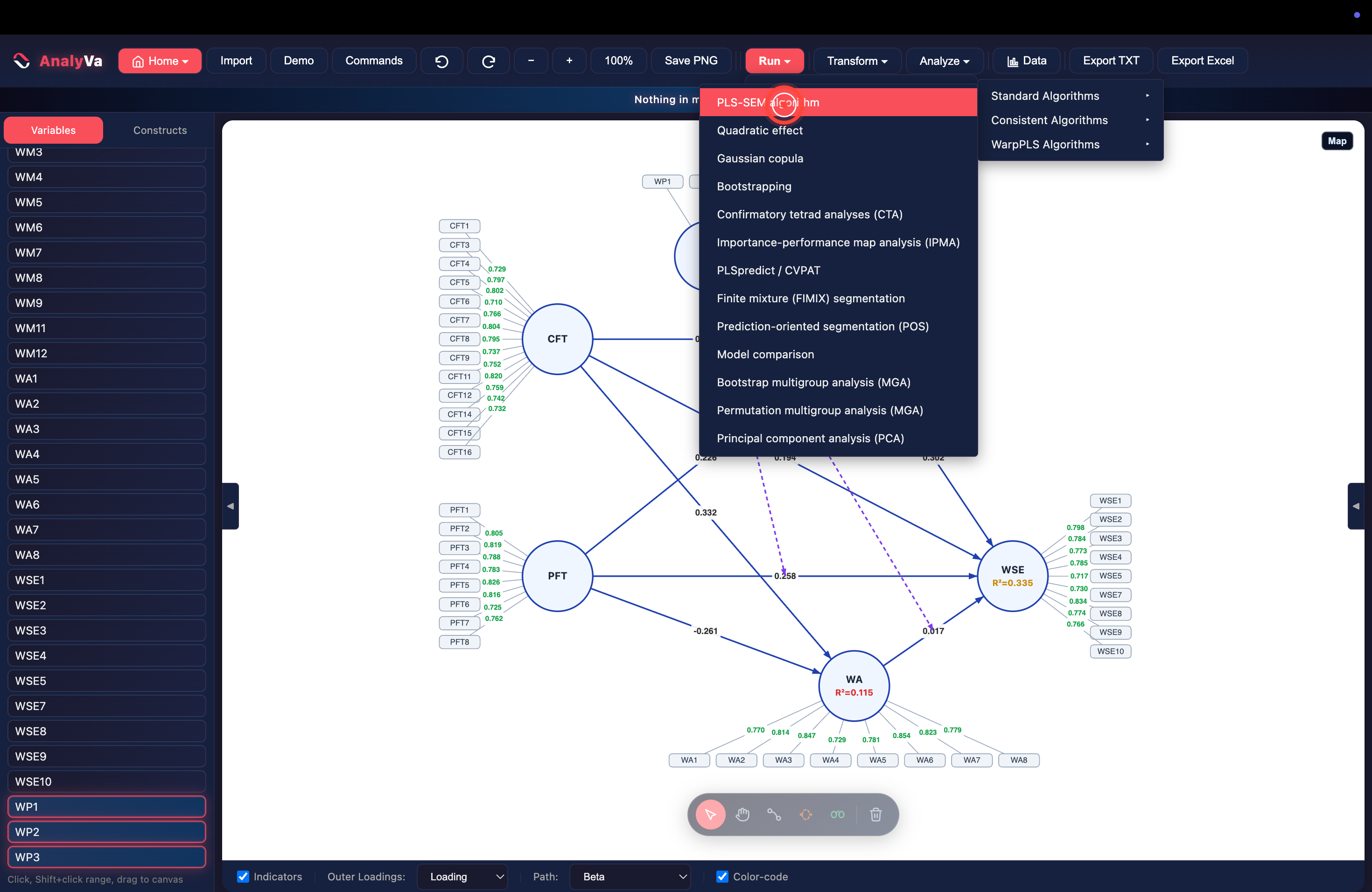
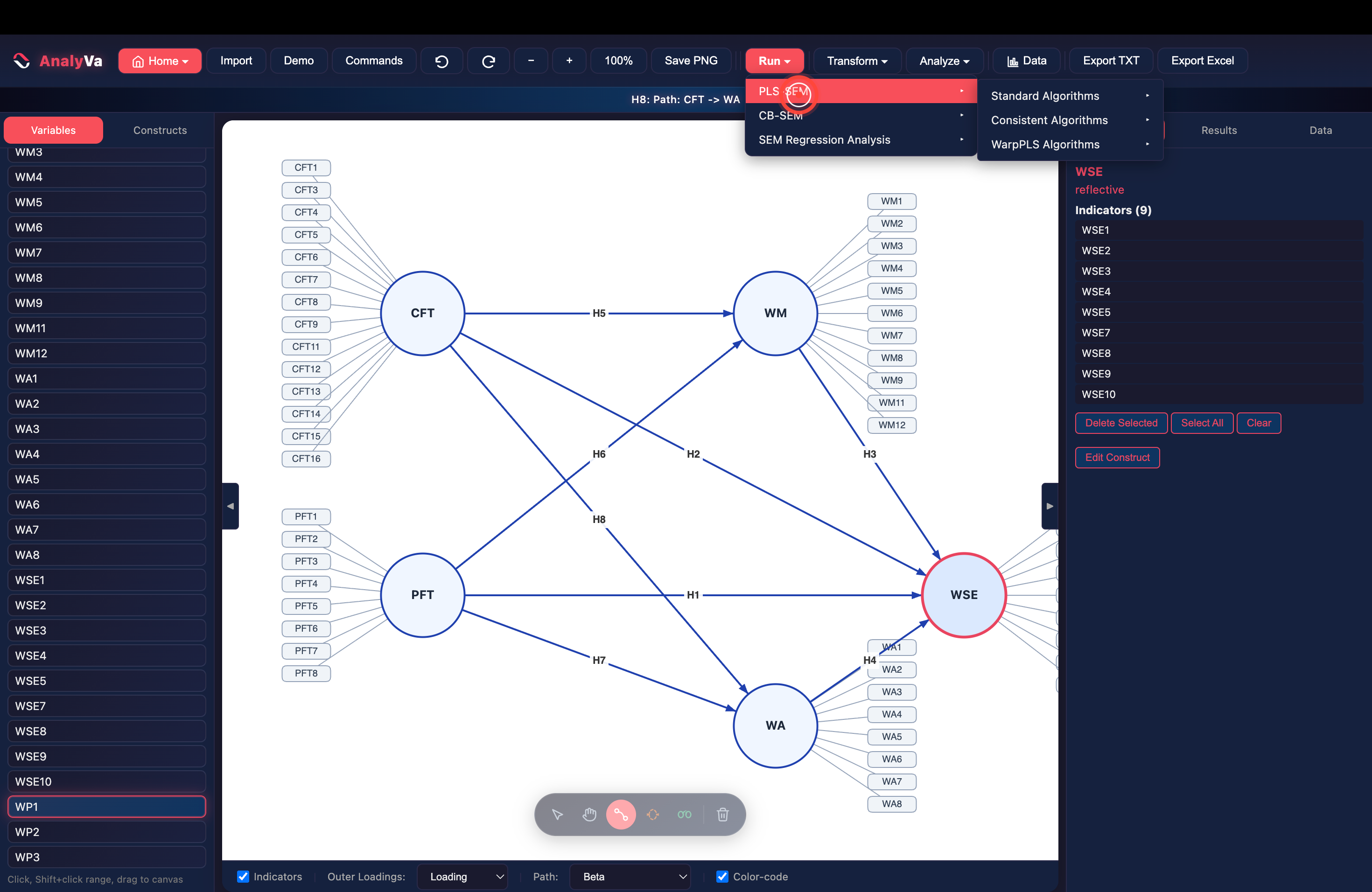
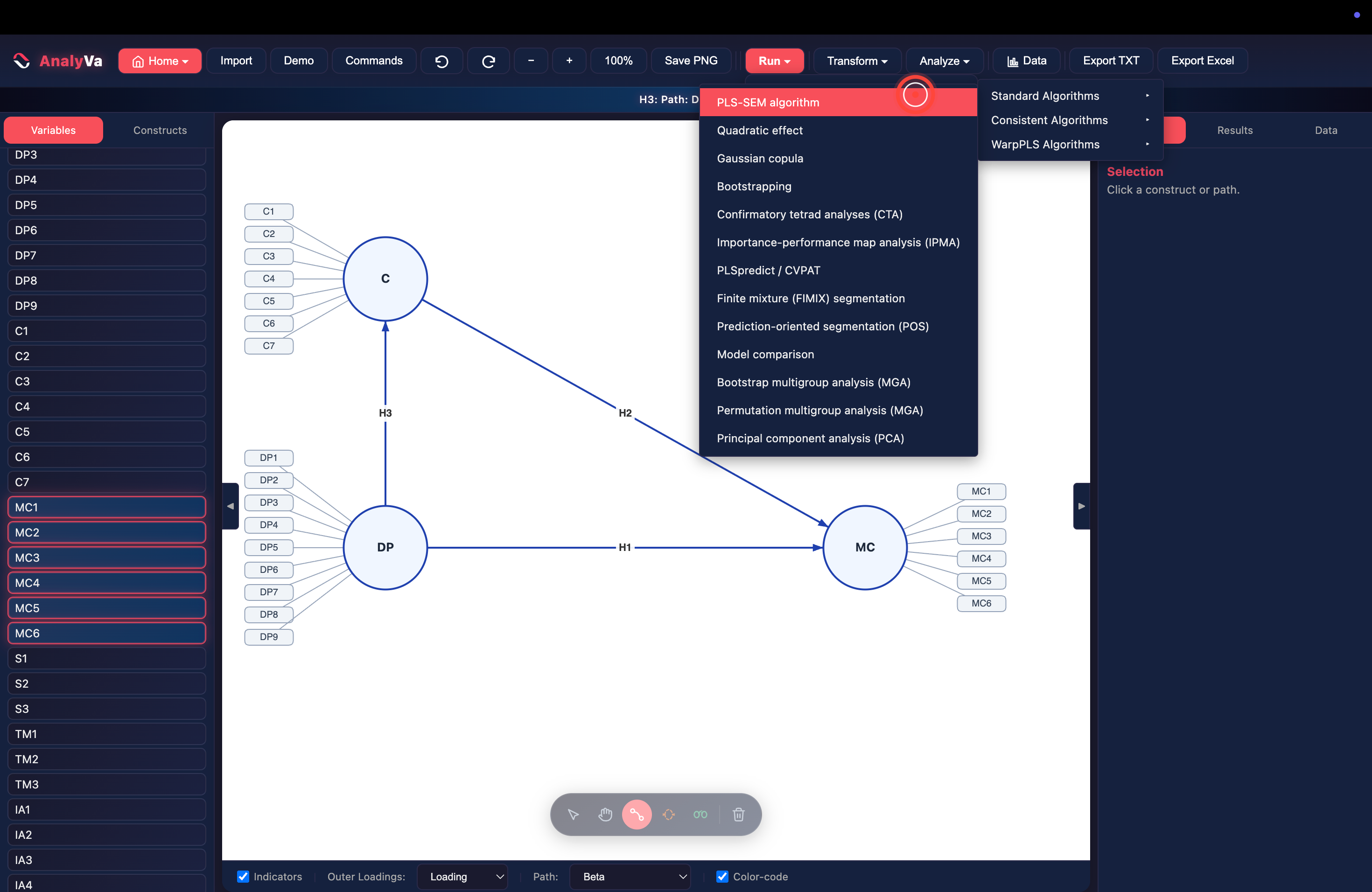
<p><strong>Step 7 — Open <em>Run → PLS-SEM → Standard Algorithms → PLS-SEM
algorithm</em> again.</strong>
The same menu used to run the base model in the earlier post — running
it again re-estimates with the four new interaction terms included.</p>

<p><img src="/blog/images/analyva-moderation-07.png" alt="The PLS-SEM submenu reopened with the moderated model on canvas" /></p>

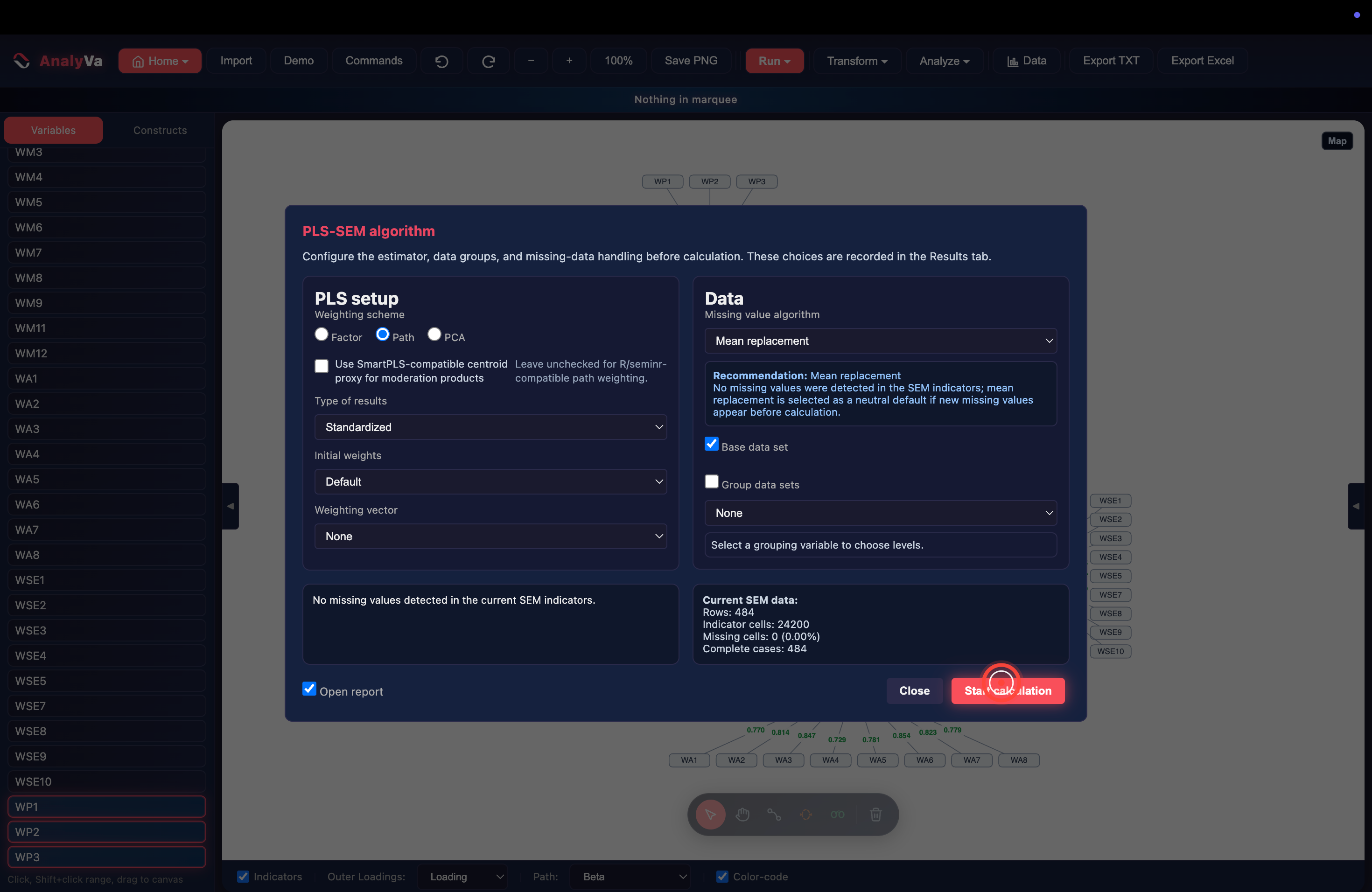
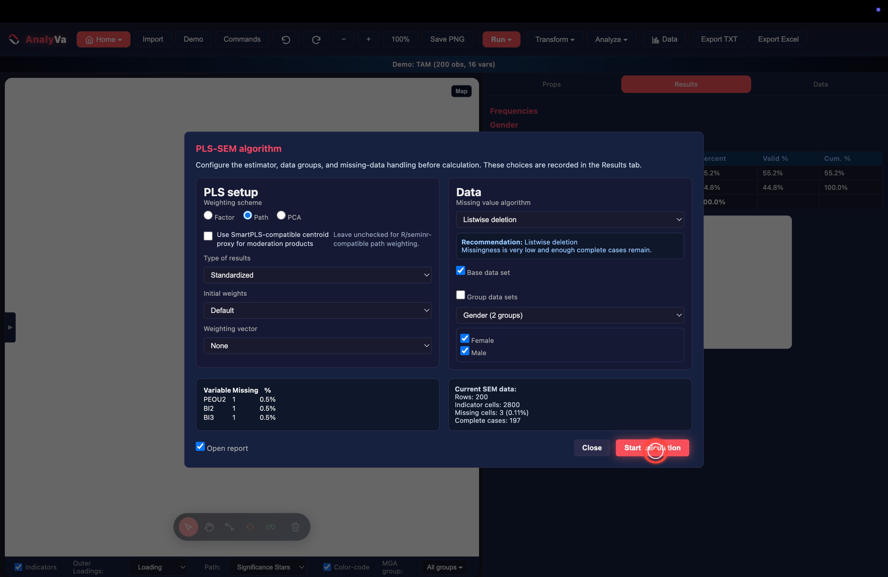
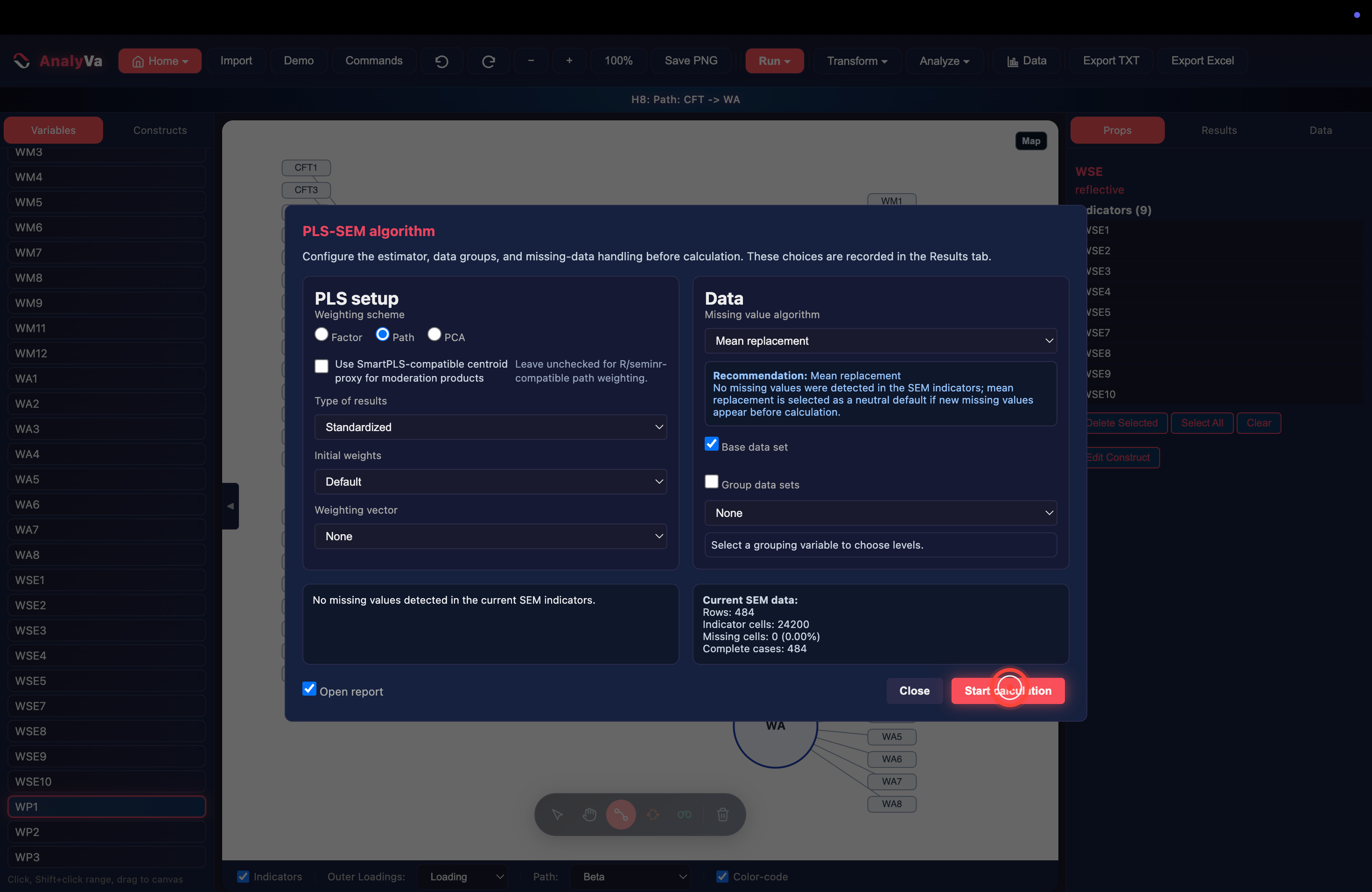
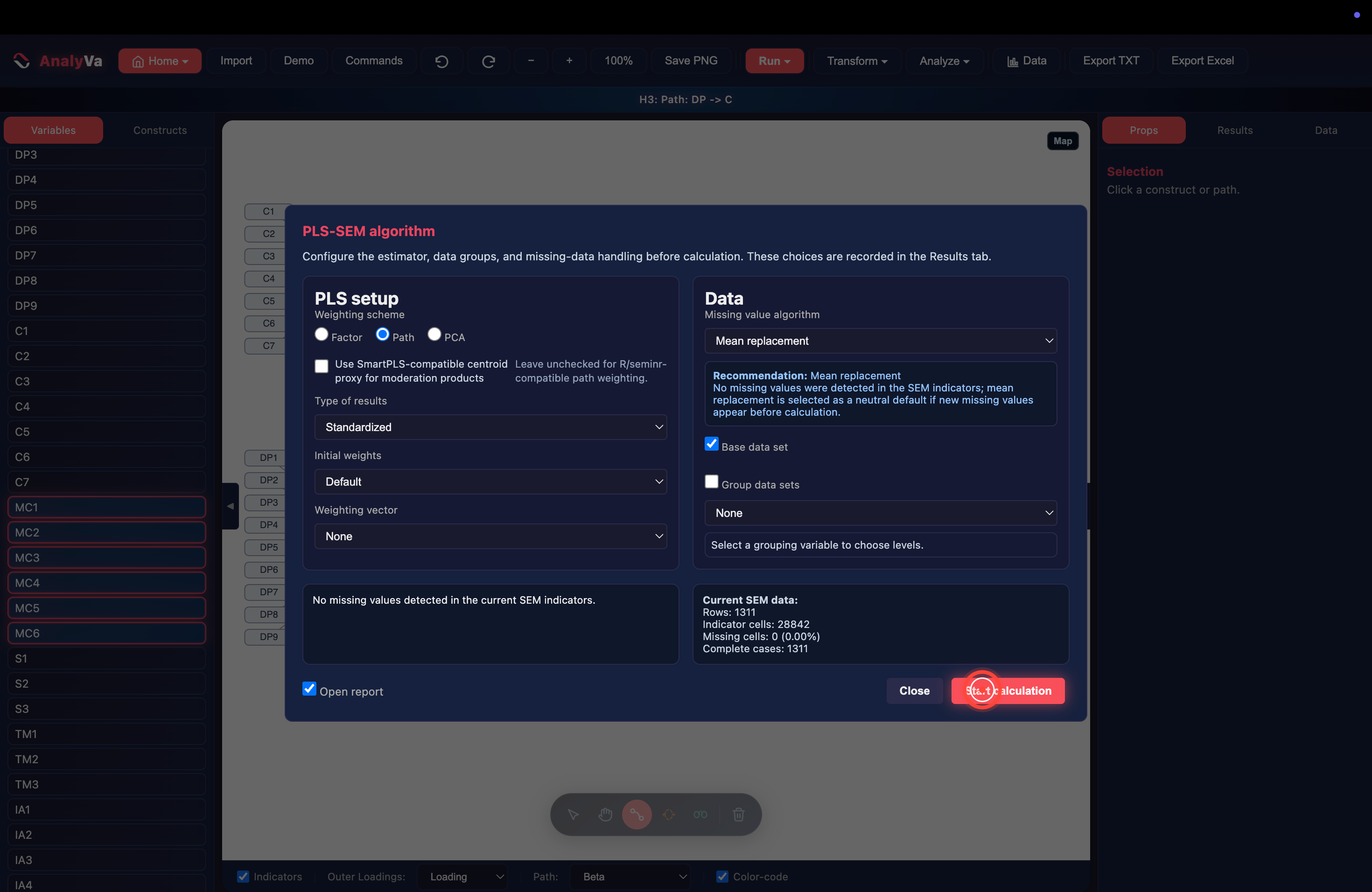
<p><strong>Step 8 — Check the moderation-specific setup option, then start.</strong>
The configuration dialog has the same Path/Factor/PCA weighting choice
as before, plus one option that only matters for moderation models:
<strong>Use SmartPLS-compatible centroid proxy for moderation products.</strong>
Leaving it unchecked matches R/seminr-style path weighting; checking it
matches SmartPLS’s centroid approach for building interaction terms.
Pick whichever matches the software you’re benchmarking against, then
click <strong>Start calculation</strong>.</p>

<p><img src="/blog/images/analyva-moderation-08.png" alt="The PLS-SEM algorithm dialog with the SmartPLS-compatible centroid checkbox for moderation products" /></p>

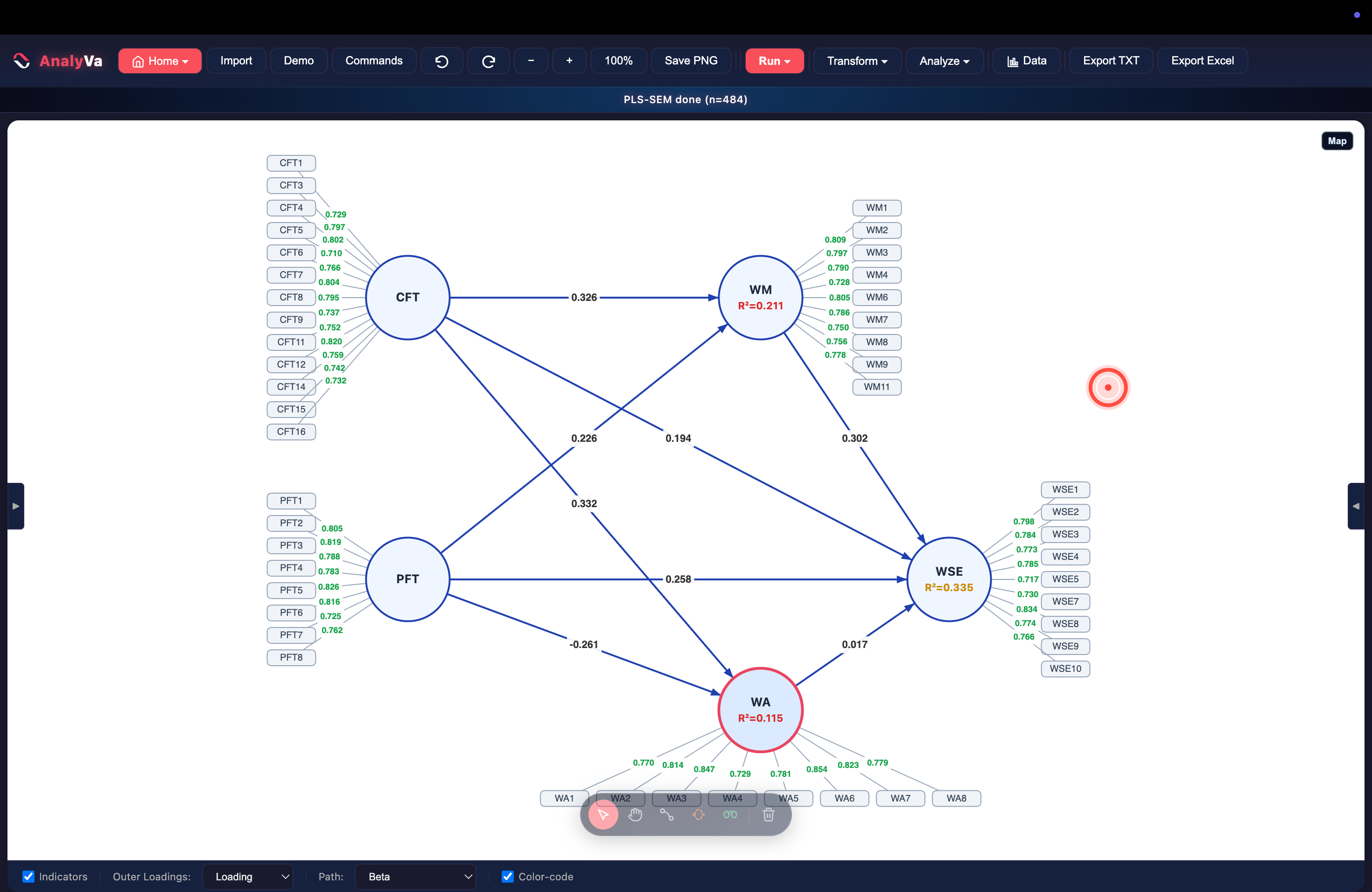
<p>Adding the moderator changes the outcome construct’s explanatory power:
WSE’s R² moves from 0.335 in the unmoderated model to <strong>0.366</strong> here —
the four interaction terms and WP’s direct effect together account for
that gain.</p>

<h2 id="bootstrapping-for-significance">Bootstrapping for significance</h2>

<p>Path coefficients alone don’t tell you which moderation effects are
real. That requires bootstrapping.</p>

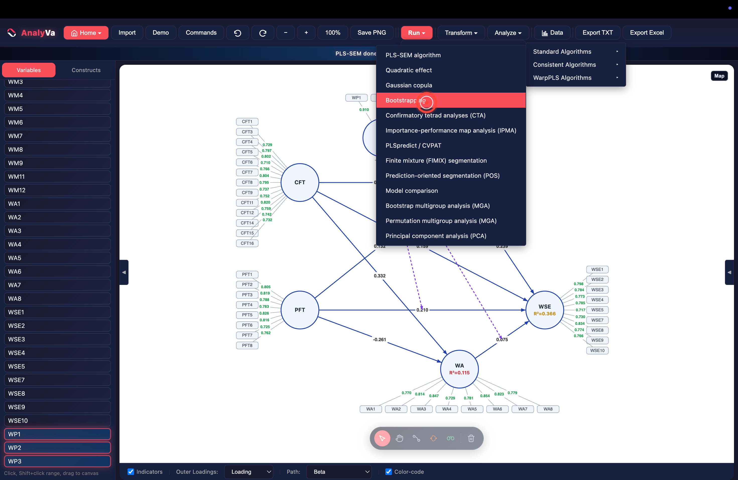
<p><strong>Step 9 — Open <em>Run → PLS-SEM → Bootstrapping</em>.</strong></p>

<p><img src="/blog/images/analyva-moderation-09.png" alt="Run menu open with Bootstrapping highlighted, moderated model already estimated" /></p>

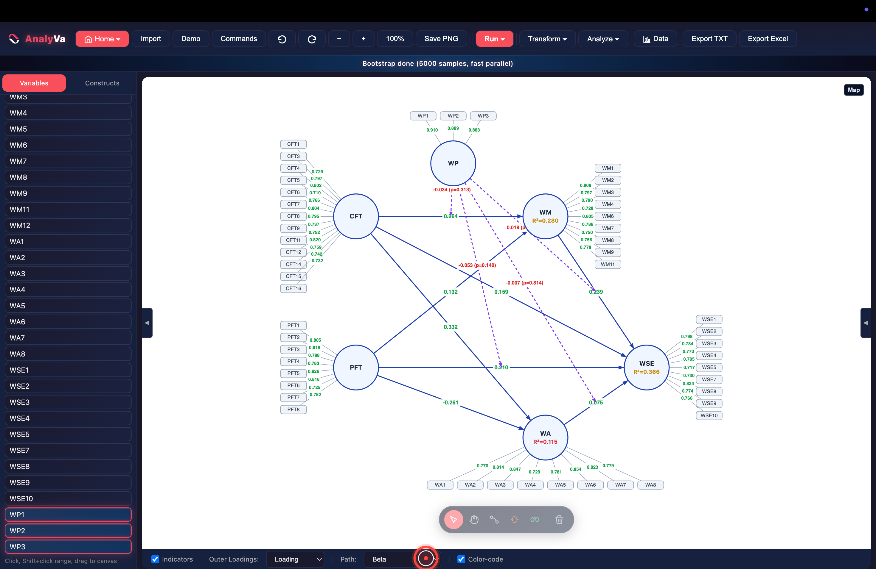
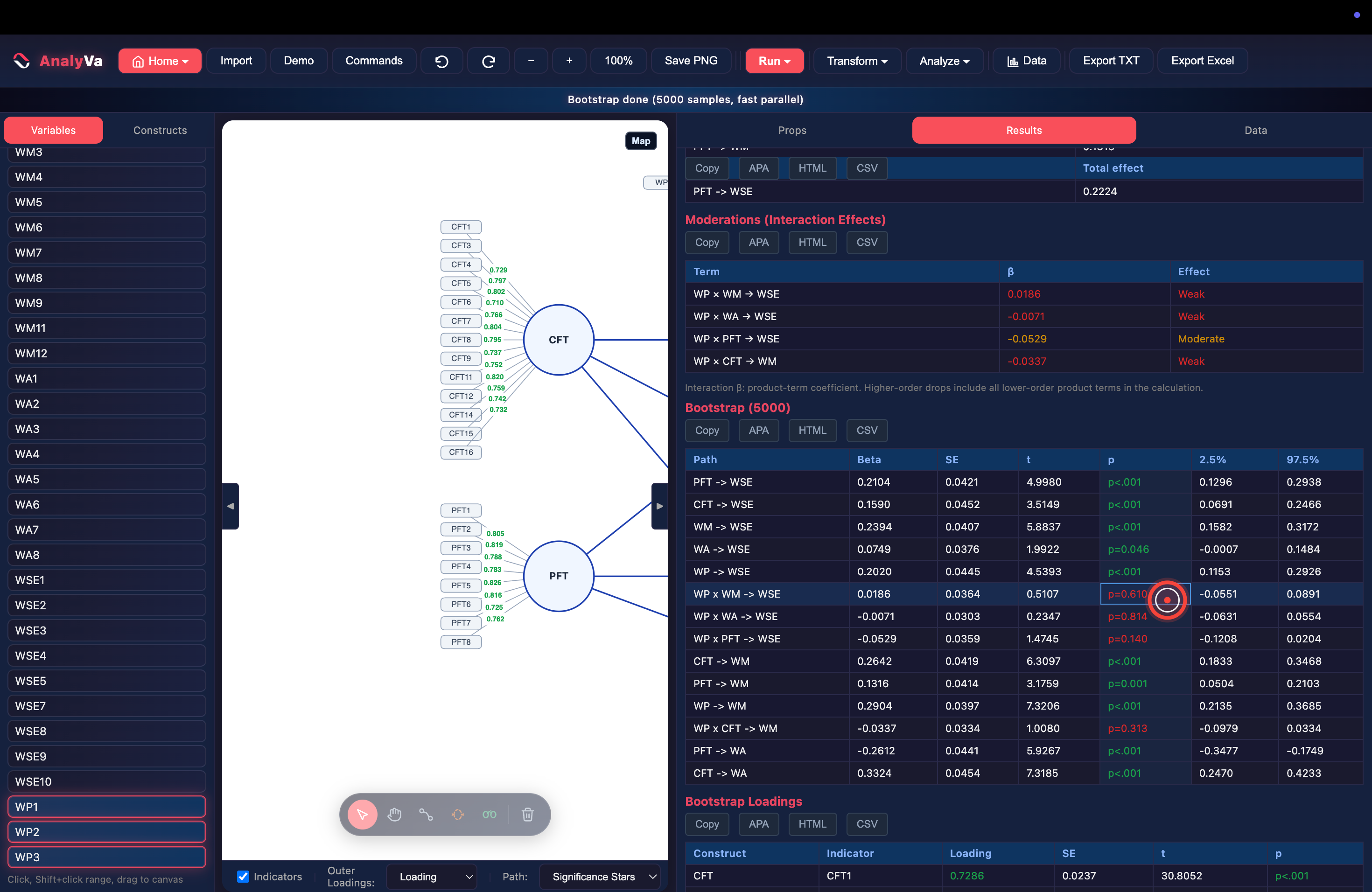
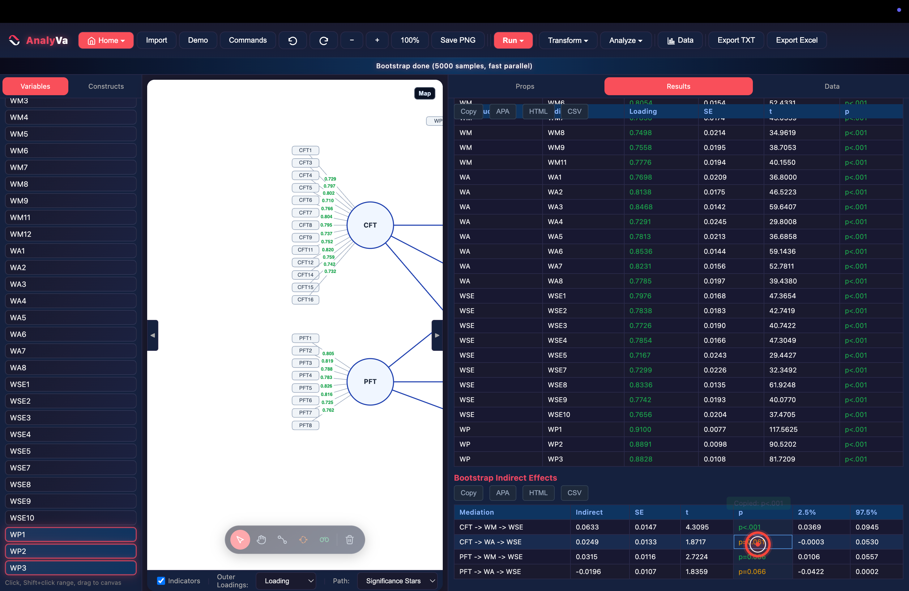
<p><strong>Step 10 — Read the Beta (p) display.</strong>
AnalyVa runs 5,000 bootstrap resamples (<em>“fast parallel”</em>) and, by
default, annotates each path with its coefficient and p-value inline:
<code class="language-plaintext highlighter-rouge">-0.034 (p=0.313)</code>, <code class="language-plaintext highlighter-rouge">-0.053 (p=0.140)</code>, <code class="language-plaintext highlighter-rouge">-0.007 (p=0.814)</code> — all three
visible interaction terms here are non-significant at conventional
thresholds.</p>

<p><img src="/blog/images/analyva-moderation-10.png" alt="The bootstrapped model with Beta (p) values shown inline on each path" /></p>

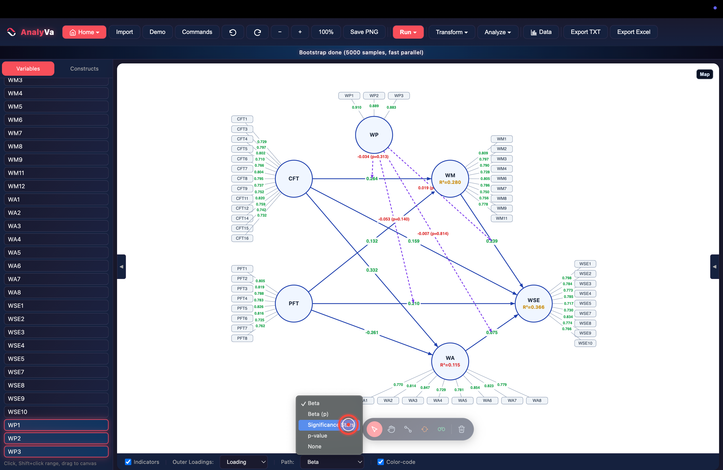
<p><strong>Step 11 — Switch the <em>Path</em> display to Significance Stars.</strong>
The dropdown at the bottom toolbar controls how path values render:
<strong>Beta</strong>, <strong>Beta (p)</strong>, <strong>Significance Stars</strong>, <strong>p-value</strong>, or
<strong>None</strong>. Switching to Significance Stars trades exact p-values for a
faster visual scan — useful once you already know roughly where the
interesting cases are.</p>

<p><img src="/blog/images/analyva-moderation-11.png" alt="The Path display dropdown open, Significance Stars selected" /></p>

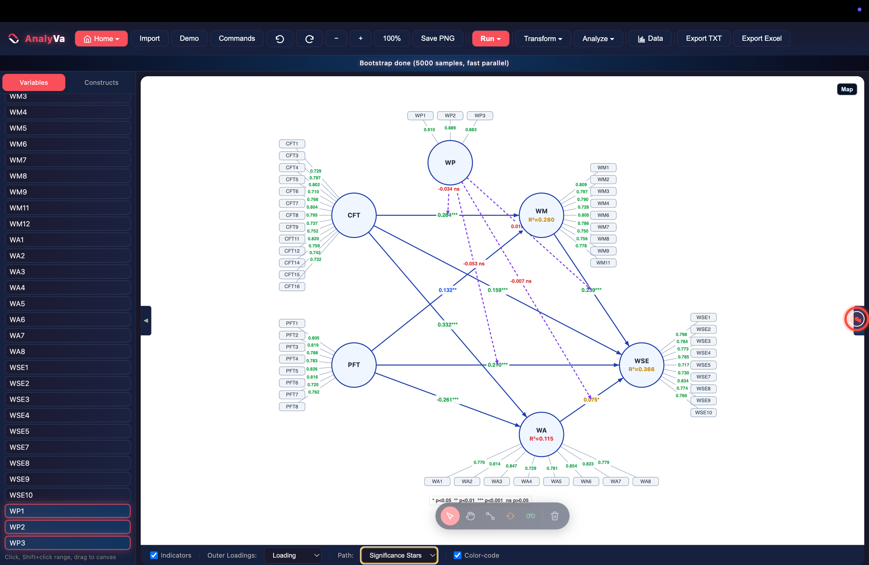
<p><strong>Step 12 — Read the starred diagram.</strong>
Every path now carries <code class="language-plaintext highlighter-rouge">***</code>, <code class="language-plaintext highlighter-rouge">**</code>, <code class="language-plaintext highlighter-rouge">*</code>, or <code class="language-plaintext highlighter-rouge">ns</code>, with a legend at the
bottom of the canvas (<code class="language-plaintext highlighter-rouge">* p&lt;0.05  ** p&lt;0.01  *** p&lt;0.001  ns p&gt;0.05</code>).
All four interaction terms read <code class="language-plaintext highlighter-rouge">ns</code>. The direct paths — CFT → WSE,
WM → WSE, PFT → WSE — stay solidly significant at <code class="language-plaintext highlighter-rouge">***</code>.</p>

<p><img src="/blog/images/analyva-moderation-12.png" alt="The full model with significance stars on every path and the legend visible" /></p>

<h2 id="reading-the-moderation-table">Reading the moderation table</h2>

<p>Stars on the canvas are a summary. The Results panel has the full
picture.</p>

<p><strong>Step 13 — Open the <em>Moderations (Interaction Effects)</em> table.</strong>
Below the standard bootstrap output, AnalyVa groups the four
interaction terms into their own table with a plain-language effect
label:</p>

<table>
  <thead>
    <tr>
      <th>Term</th>
      <th>β</th>
      <th>Effect</th>
    </tr>
  </thead>
  <tbody>
    <tr>
      <td>WP × WM → WSE</td>
      <td>0.0186</td>
      <td>Weak</td>
    </tr>
    <tr>
      <td>WP × WA → WSE</td>
      <td>−0.0071</td>
      <td>Weak</td>
    </tr>
    <tr>
      <td>WP × PFT → WSE</td>
      <td>−0.0529</td>
      <td>Moderate</td>
    </tr>
    <tr>
      <td>WP × CFT → WM</td>
      <td>−0.0337</td>
      <td>Weak</td>
    </tr>
  </tbody>
</table>

<p>None of the four reach a large effect size, and — cross-referencing the
bootstrap table below — none reach significance either (p = 0.610,
0.814, 0.140, and 0.313 respectively). That’s a real, reportable
result: this moderator doesn’t meaningfully change any of the four
paths tested, at least not in this sample.</p>

<p><img src="/blog/images/analyva-moderation-13.png" alt="The Moderations (Interaction Effects) table with beta and Weak/Moderate labels" /></p>

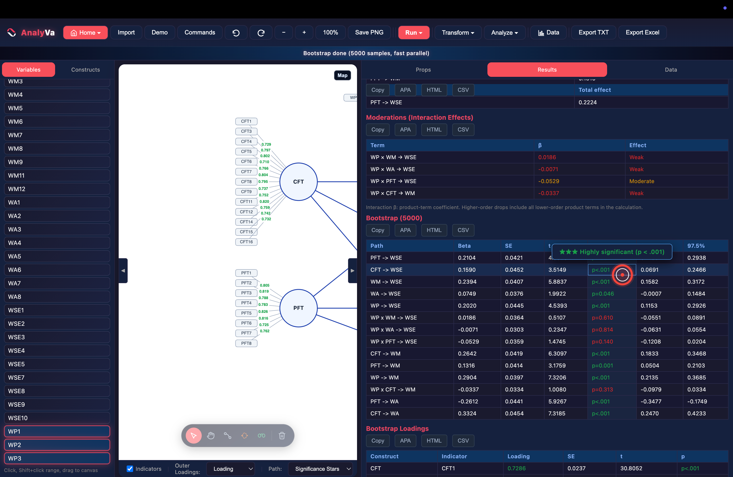
<p><strong>Step 14 — Cross-check with the full bootstrap table.</strong>
Every path — structural and interaction — gets its own row with Beta,
SE, t, p, and the 95% bootstrap confidence interval. Hovering any <code class="language-plaintext highlighter-rouge">p</code>
cell surfaces a plain-language tooltip (<em>“★★★ Highly significant
(p &lt; .001)”</em>), which is a fast way to explain a results table to a
co-author who doesn’t read t-statistics fluently.</p>

<p><img src="/blog/images/analyva-moderation-14.png" alt="The full bootstrap results table with a hover tooltip reading Highly significant" /></p>

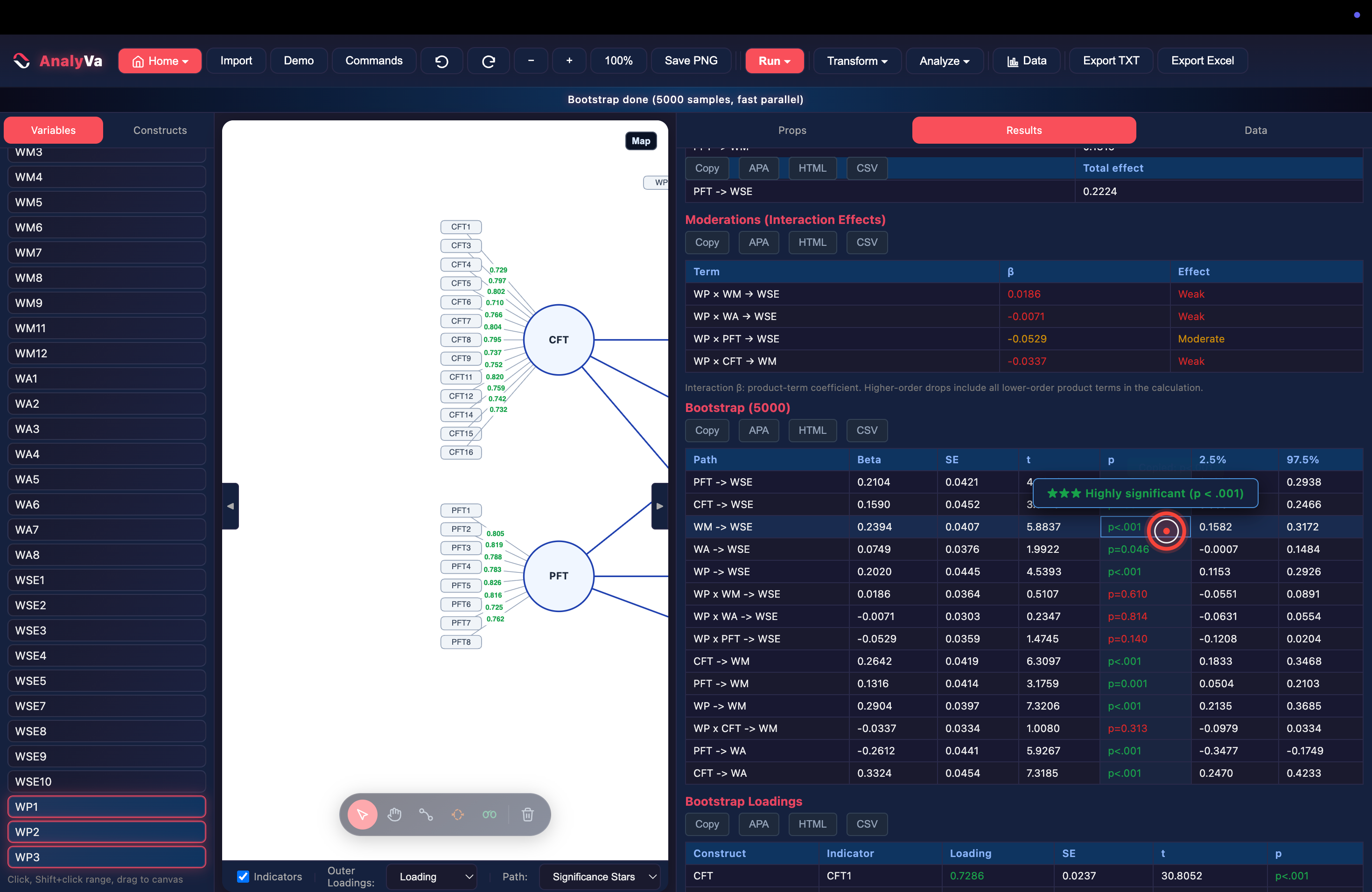
<p><strong>Step 15 — Note which paths are genuinely significant.</strong>
The base structural paths (PFT → WSE, CFT → WSE, WM → WSE, WP → WSE,
CFT → WM, PFT → WM, WP → WM) all clear <code class="language-plaintext highlighter-rouge">p&lt;.001</code>. Only the interaction
terms are the non-significant group here — a pattern worth stating
explicitly in a manuscript: <em>“the direct effects held; none of the
four hypothesized moderations were supported.”</em></p>

<p><img src="/blog/images/analyva-moderation-15.png" alt="The bootstrap table with the highly-significant tooltip and non-significant interaction rows visible" /></p>

<h2 id="loadings-and-indirect-effects-same-run">Loadings and indirect effects, same run</h2>

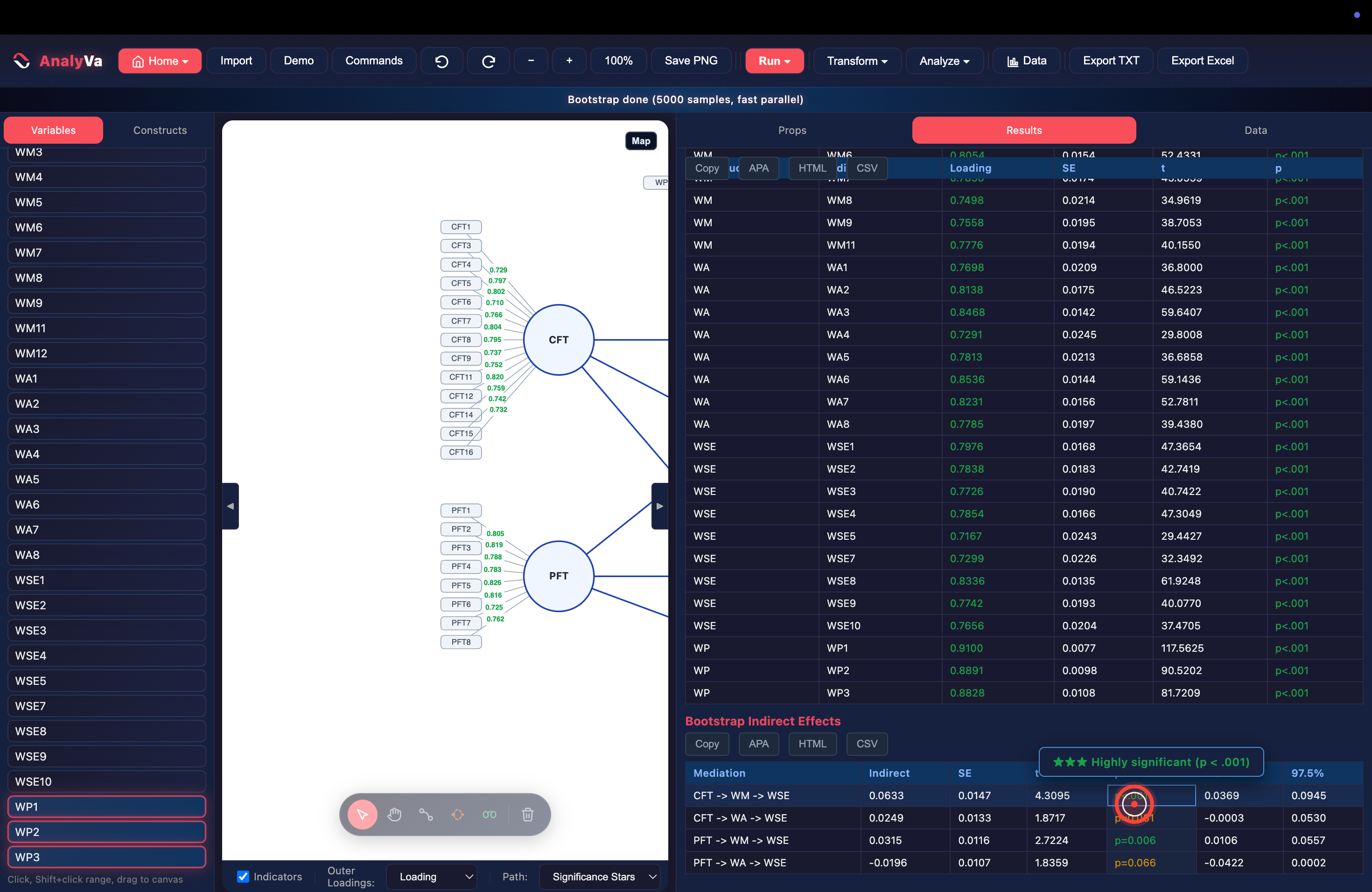
<p><strong>Step 16 — Scroll to Bootstrap Loadings.</strong>
The same 5,000-sample bootstrap also re-estimates every outer loading
with its own SE, t, and p — every indicator here clears <code class="language-plaintext highlighter-rouge">p&lt;.001</code>.</p>

<p><img src="/blog/images/analyva-moderation-16.png" alt="Bootstrap Loadings table listing every indicator with SE, t, and p" /></p>

<p><strong>Step 17 — Check Bootstrap Indirect Effects for mediation.</strong>
Because CFT and PFT both route through WM and WA on their way to WSE,
AnalyVa also reports the indirect (mediated) effect for each path —
CFT → WM → WSE, CFT → WA → WSE, PFT → WM → WSE, PFT → WA → WSE — with
its own confidence interval. This comes free in the same run; no
separate mediation analysis needed.</p>

<p><img src="/blog/images/analyva-moderation-17.png" alt="Bootstrap Indirect Effects table showing four mediation paths with confidence intervals" /></p>

<h2 id="what-to-report">What to report</h2>

<p>A null moderation result is still a result. The write-up here would
state: R² for WSE improved marginally with the moderator added (0.335
→ 0.366), but all four interaction terms were non-significant under
5,000-sample bootstrapping (p &gt; 0.10 in every case), so the hypothesis
that WP moderates these relationships is not supported in this sample.
That’s a defensible, complete finding — and every number needed to
write it came out of a single PLS-SEM run plus one bootstrap pass.</p>]]></content><author><name>Abdelouahd Bouzar</name><email>support@analyva.com</email></author><category term="PLS-SEM" /><category term="analyva" /><category term="pls-sem" /><category term="moderation" /><category term="bootstrapping" /><summary type="html"><![CDATA[Add a moderator construct to an existing PLS-SEM model, draw four interaction paths, run the SmartPLS-compatible centroid estimator, and read significance with bootstrap stars instead of raw p-values.]]></summary><media:thumbnail xmlns:media="http://search.yahoo.com/mrss/" url="https://analyva.com/blog/images/cover-moderation.svg" /><media:content medium="image" url="https://analyva.com/blog/images/cover-moderation.svg" xmlns:media="http://search.yahoo.com/mrss/" /></entry><entry><title type="html">Recoding a Variable into Groups and Running Multi-Group Analysis</title><link href="https://analyva.com/blog/recode-variables-for-multi-group-analysis/" rel="alternate" type="text/html" title="Recoding a Variable into Groups and Running Multi-Group Analysis" /><published>2026-08-06T00:00:00+00:00</published><updated>2026-08-06T00:00:00+00:00</updated><id>https://analyva.com/blog/recode-variables-for-multi-group-analysis</id><content type="html" xml:base="https://analyva.com/blog/recode-variables-for-multi-group-analysis/"><![CDATA[<p>Multi-group analysis (MGA) asks a simple question with a fiddly setup:
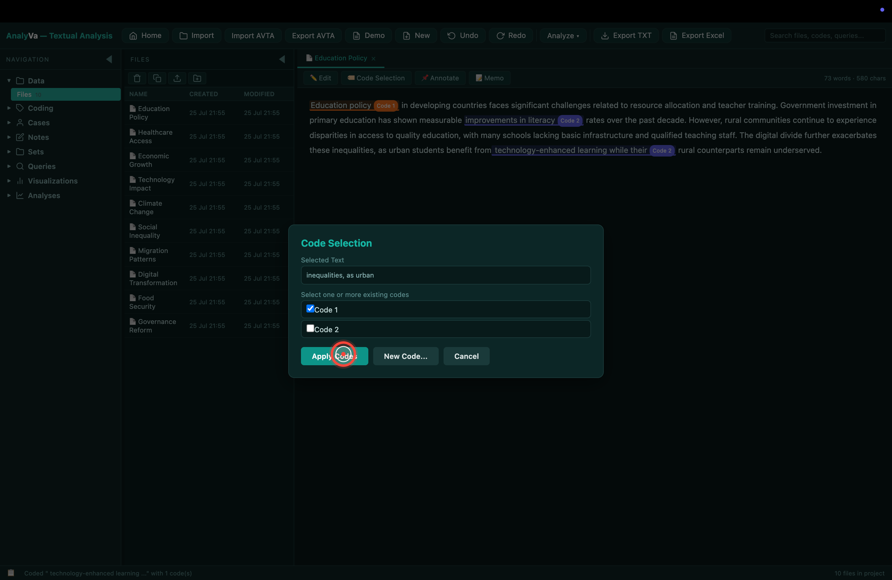
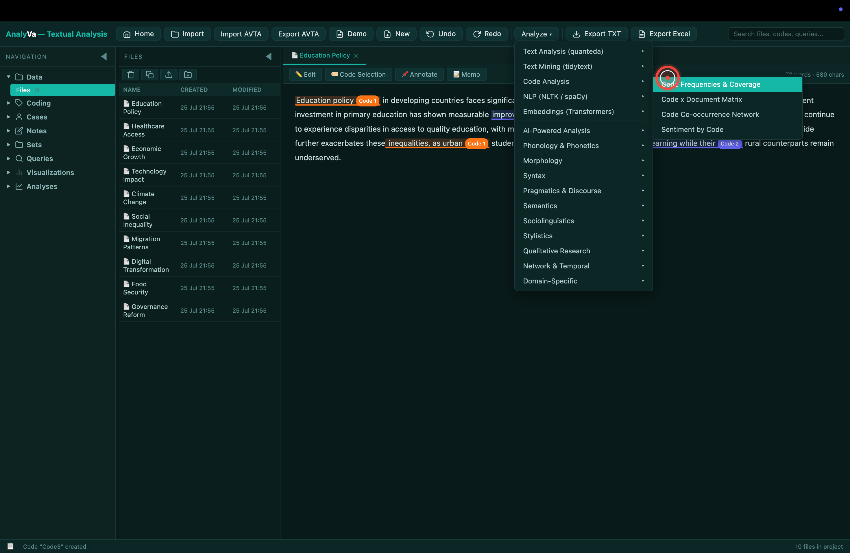
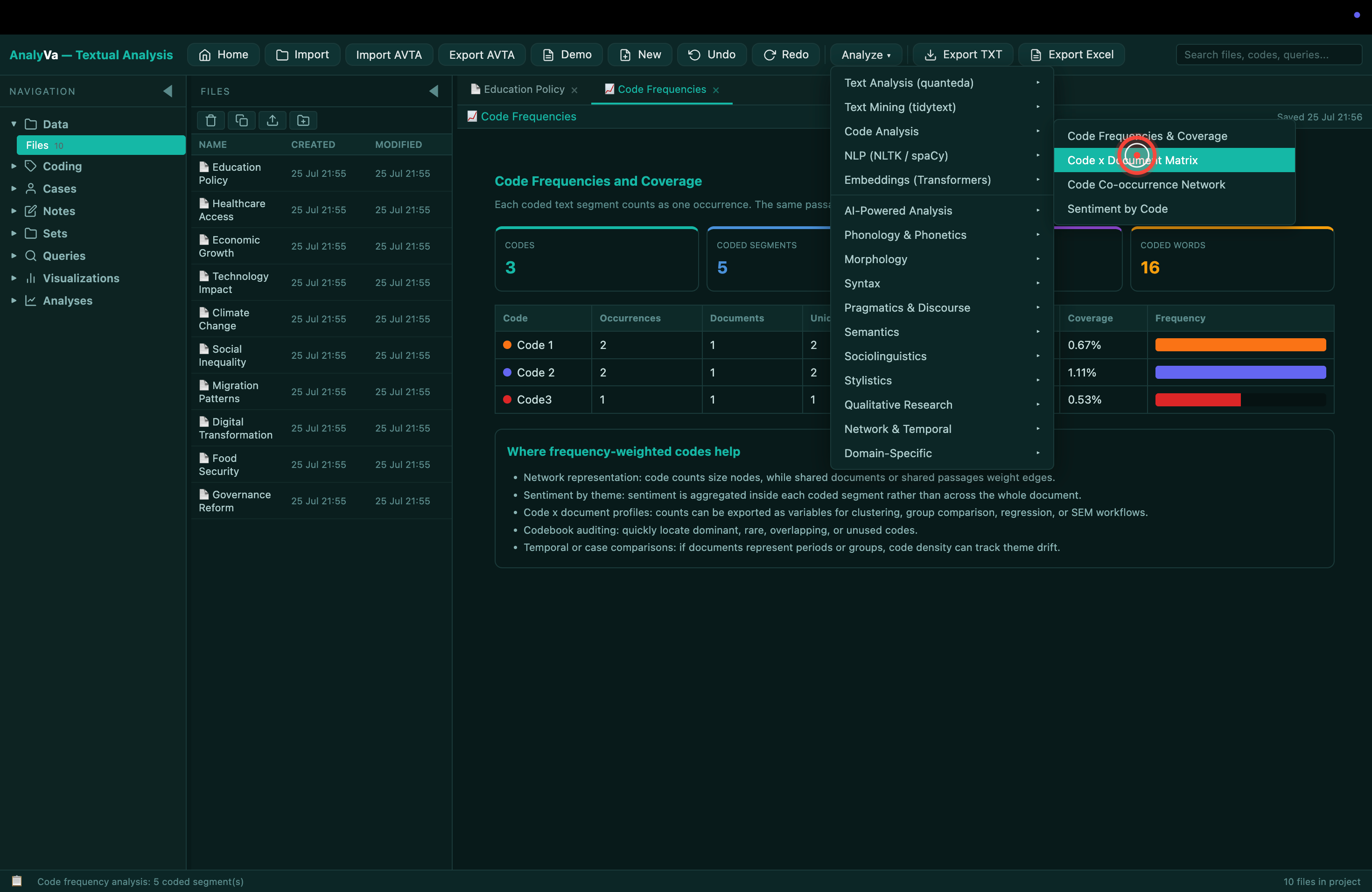
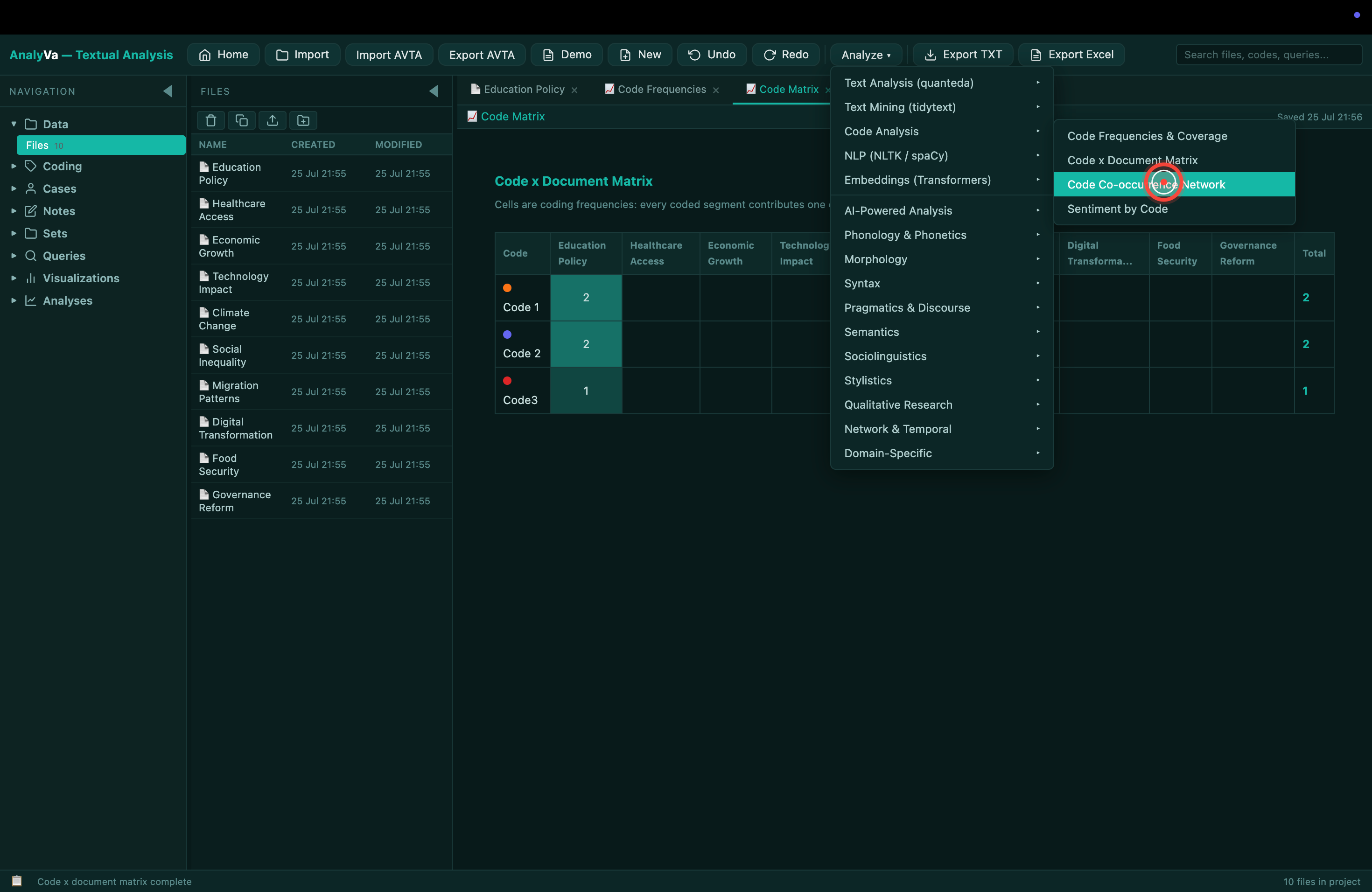
does a path coefficient differ between two groups — men and women,
novice and expert users, before and after an intervention? Before
AnalyVa can split a model by group, that grouping variable has to exist
and be labeled clearly. This post covers both halves: recoding a raw
numeric column into a labeled grouping variable, and then using it to
run an actual group comparison in the PLS-SEM dialog.</p>

<h2 id="preparing-the-grouping-variable">Preparing the grouping variable</h2>

<p>The dataset here is a 1,311-row student survey. <code class="language-plaintext highlighter-rouge">Gender</code> is already
numeric (<code class="language-plaintext highlighter-rouge">1</code> / <code class="language-plaintext highlighter-rouge">2</code>), which AnalyVa can group on directly — but labeling
it first makes every downstream table and chart readable.</p>

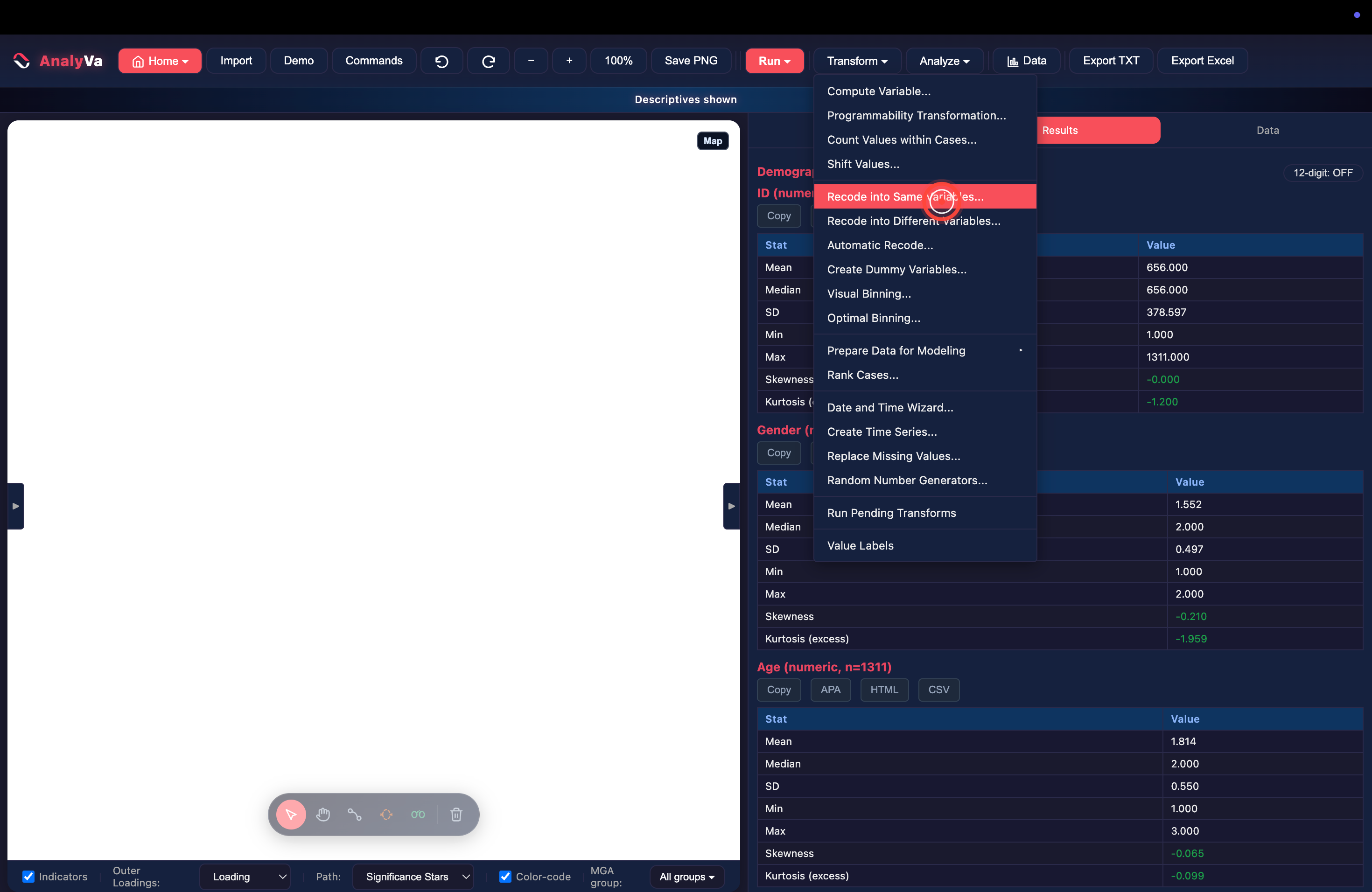
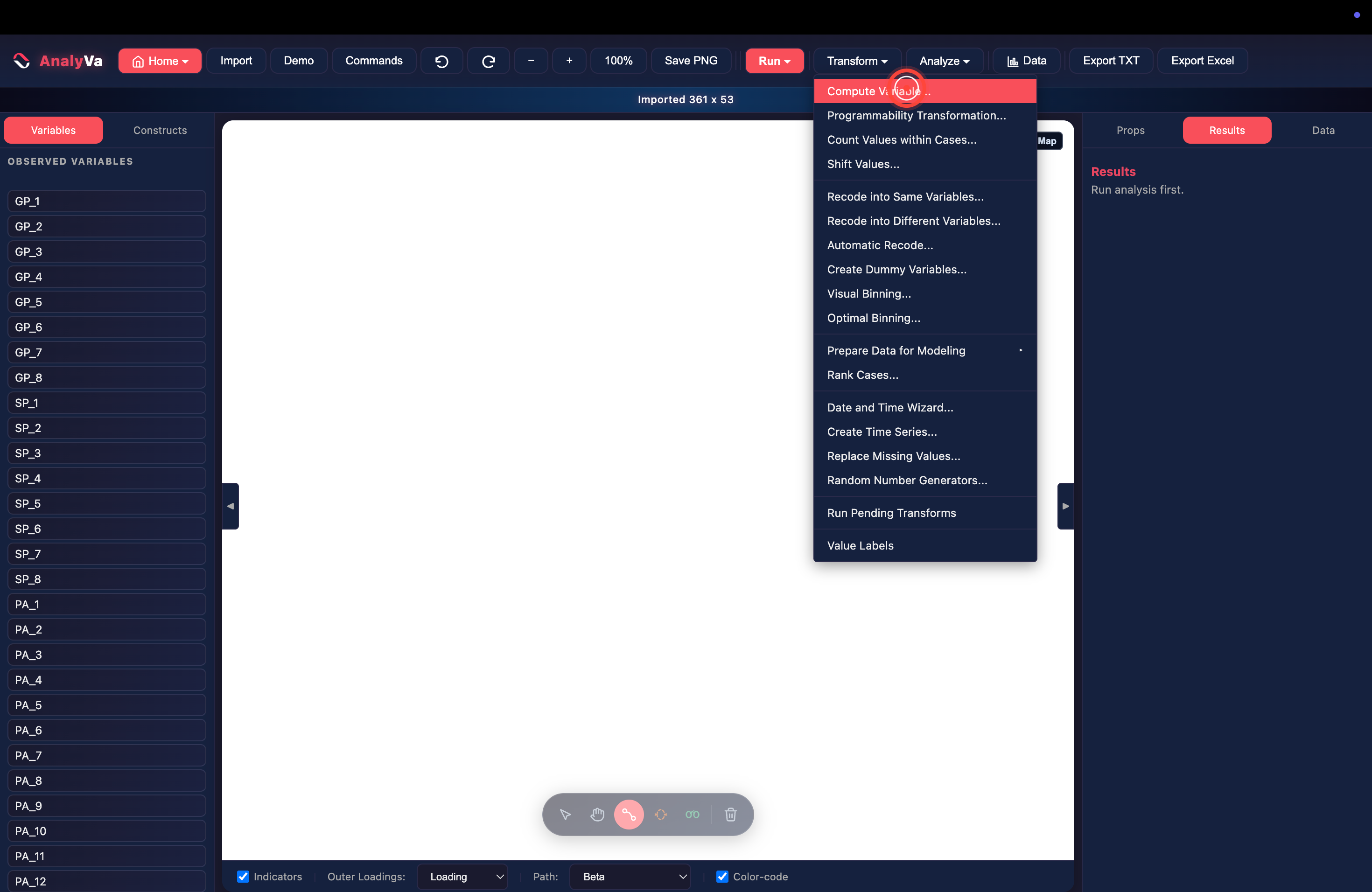
<p><strong>Step 1 — Open <em>Transform → Recode into Same Variables</em>.</strong>
With descriptives already reviewed, open the Transform menu.
<strong>Recode into Same Variables</strong> overwrites the values in place — the
right choice for turning <code class="language-plaintext highlighter-rouge">1</code>/<code class="language-plaintext highlighter-rouge">2</code> into readable labels without keeping
a duplicate column.</p>

<p><img src="/blog/images/analyva-mga-01.png" alt="Transform menu open with Recode into Same Variables highlighted" /></p>

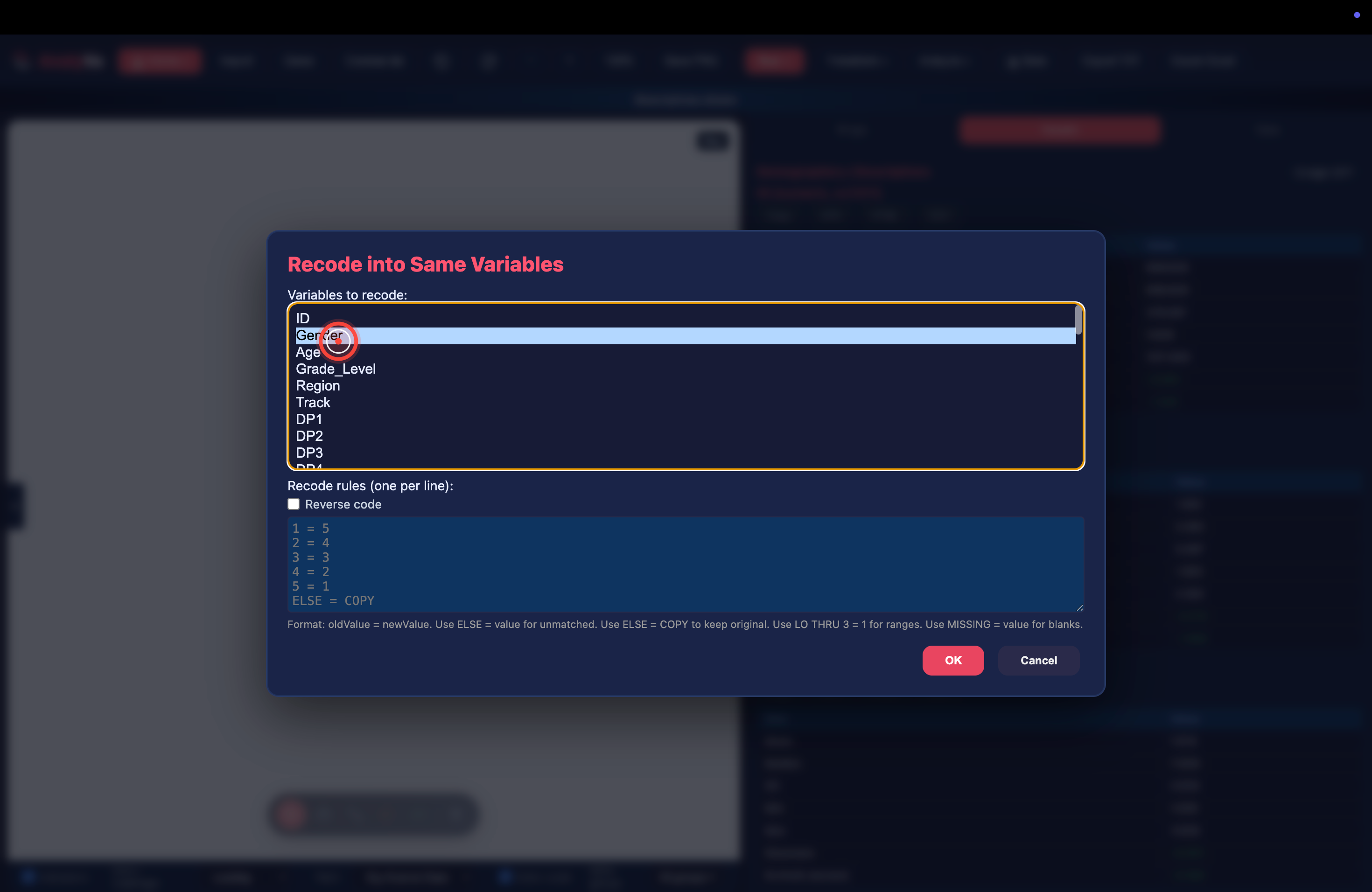
<p><strong>Step 2 — Select <em>Gender</em> from the variable list.</strong>
The dialog lists every variable in the dataset. Click <code class="language-plaintext highlighter-rouge">Gender</code>.</p>

<p><img src="/blog/images/analyva-mga-02.png" alt="Gender selected in the Recode into Same Variables dialog" /></p>

<p><strong>Step 3 — Clear the example template.</strong>
The rules box starts with placeholder text illustrating the syntax (a
5-point reverse-code example, in this case) — not the rule for this
variable. Clear it.</p>

<p><img src="/blog/images/analyva-mga-03.png" alt="The recode rules box showing the placeholder syntax example" /></p>

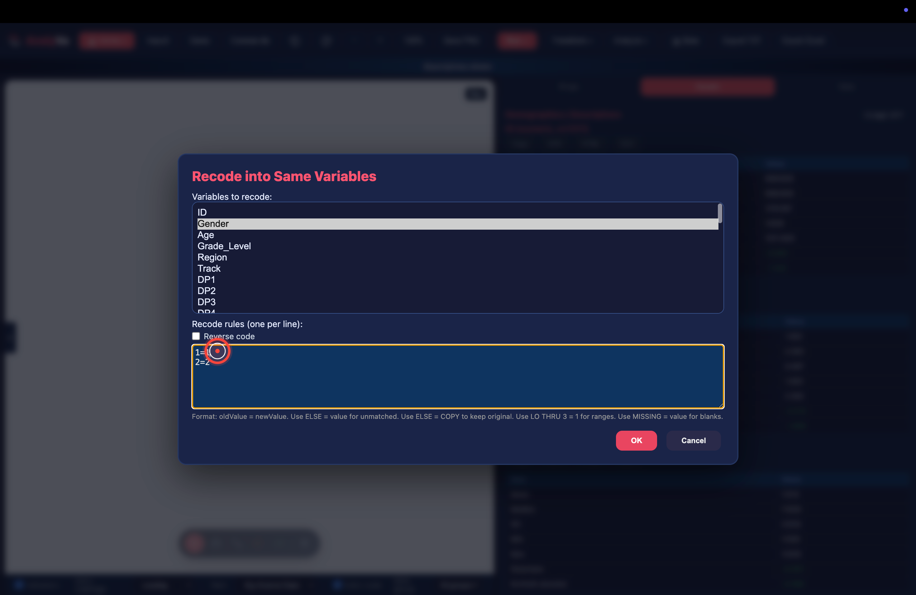
<p><strong>Step 4 — Type the actual mapping.</strong>
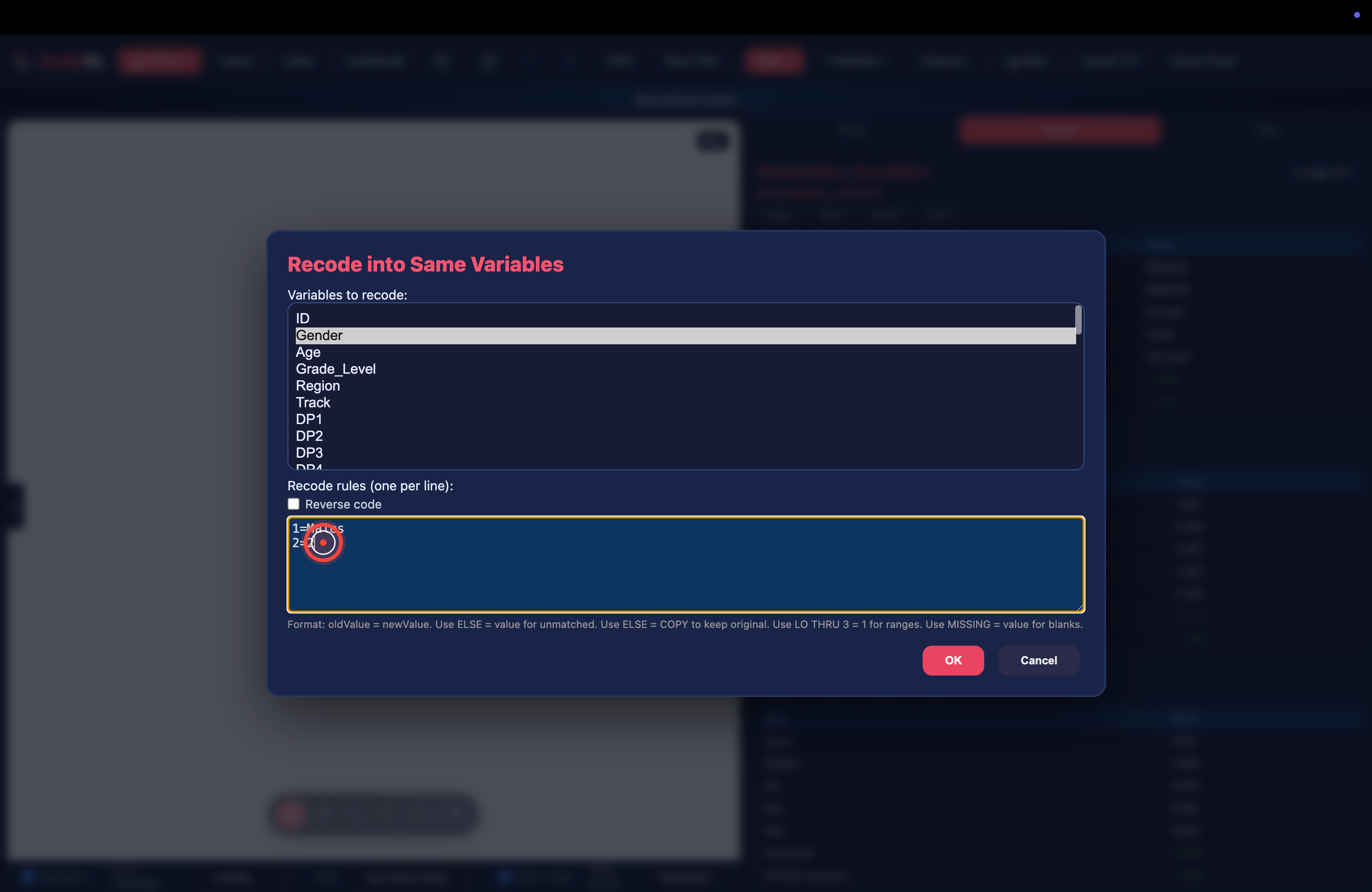
One rule per line, <code class="language-plaintext highlighter-rouge">oldValue = newValue</code>:</p>

<div class="language-plaintext highlighter-rouge"><div class="highlight"><pre class="highlight"><code>1=Males
2=Females
</code></pre></div></div>

<p><img src="/blog/images/analyva-mga-04.png" alt="The recode rules box with 1=Males and 2=Females typed in" /></p>

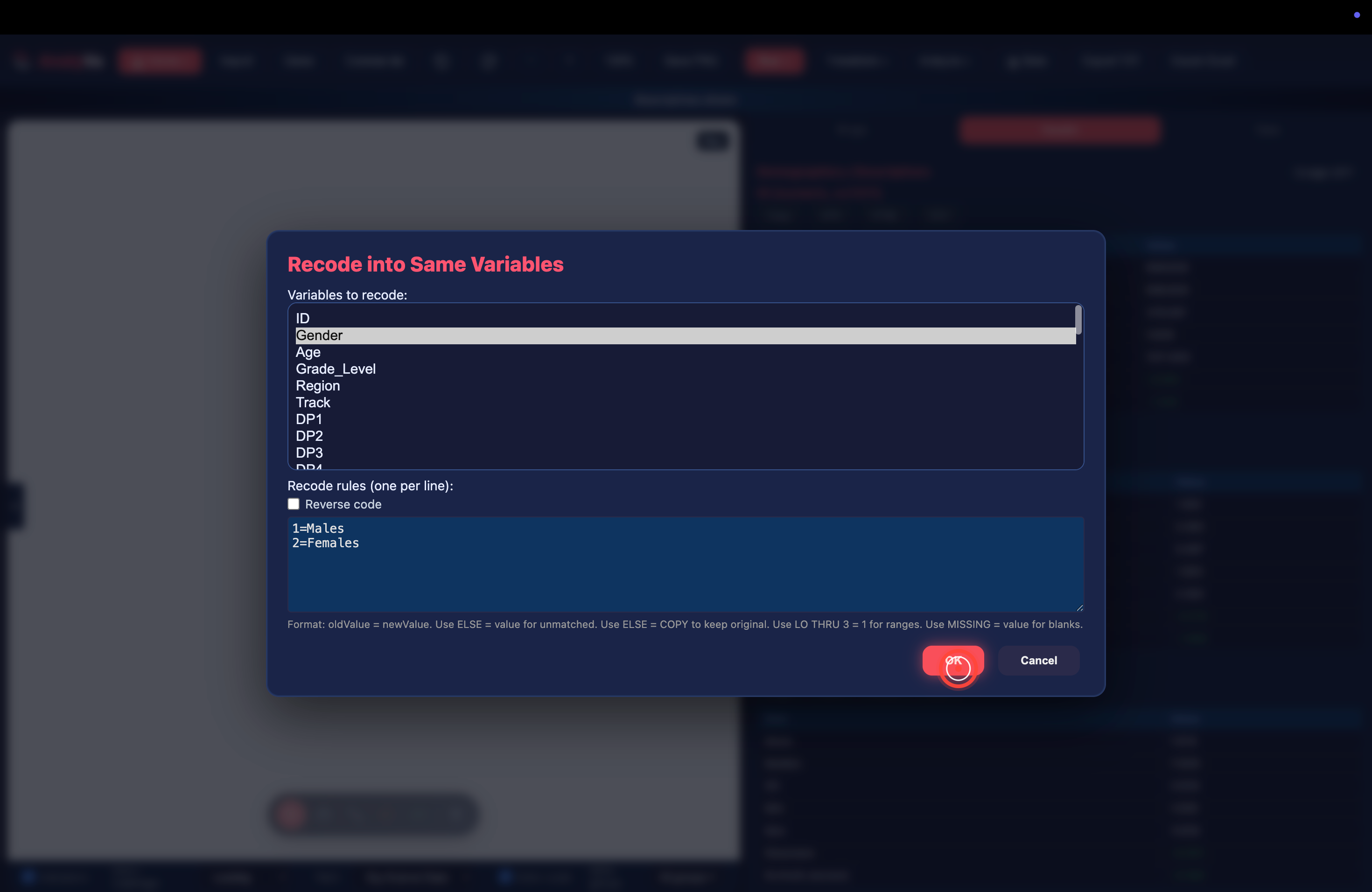
<p><strong>Step 5 — Click <em>OK</em>.</strong>
AnalyVa applies the recode in place.</p>

<p><img src="/blog/images/analyva-mga-05.png" alt="The completed recode dialog with Males/Females rules and OK highlighted" /></p>

<h2 id="verifying-the-recode">Verifying the recode</h2>

<p>Never trust a recode without checking it — a typo in the mapping
silently corrupts every downstream group comparison.</p>

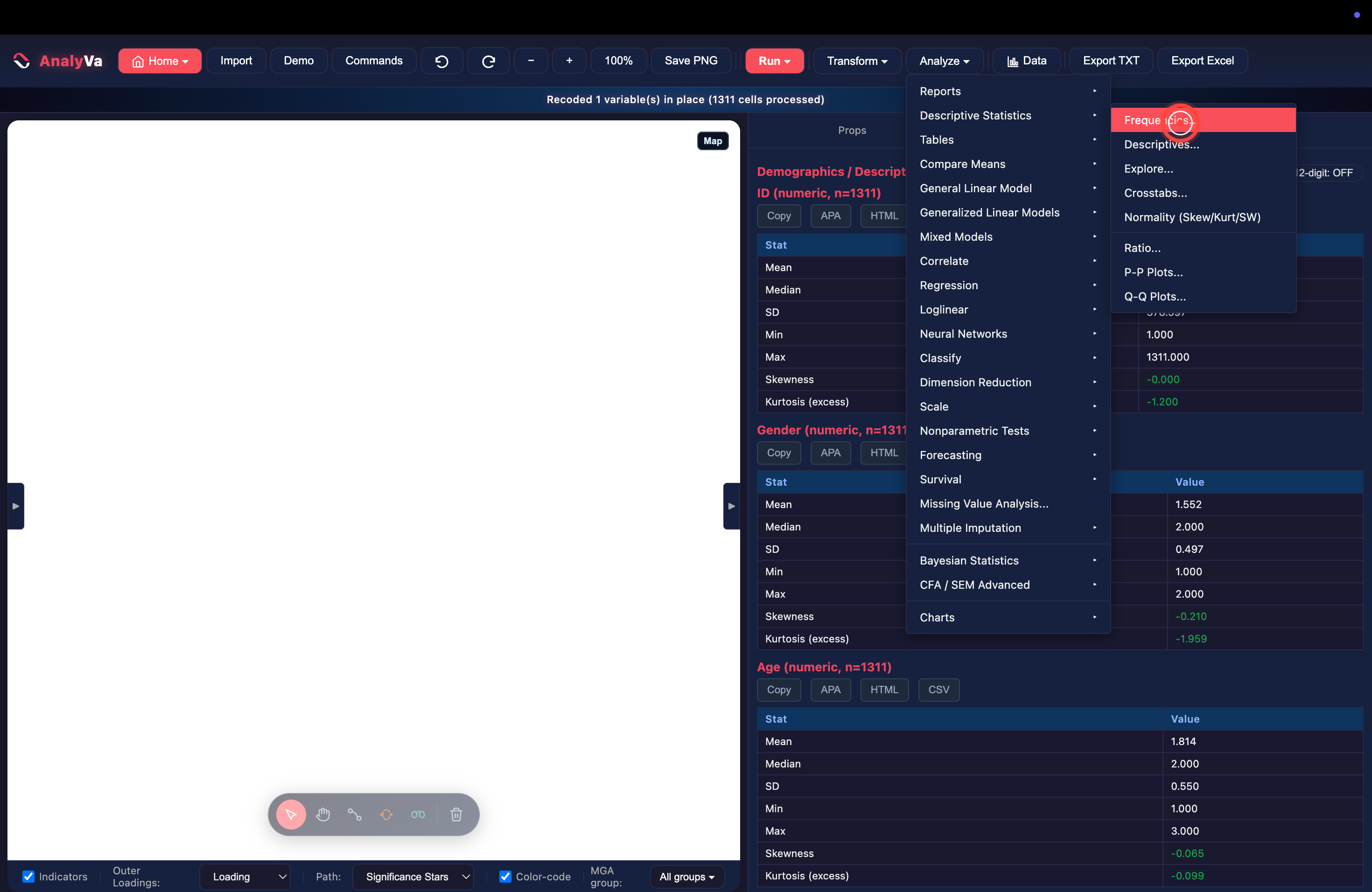
<p><strong>Step 6 — Open <em>Analyze → Descriptive Statistics → Frequencies</em>.</strong></p>

<p><img src="/blog/images/analyva-mga-06.png" alt="Analyze menu open with Frequencies highlighted" /></p>

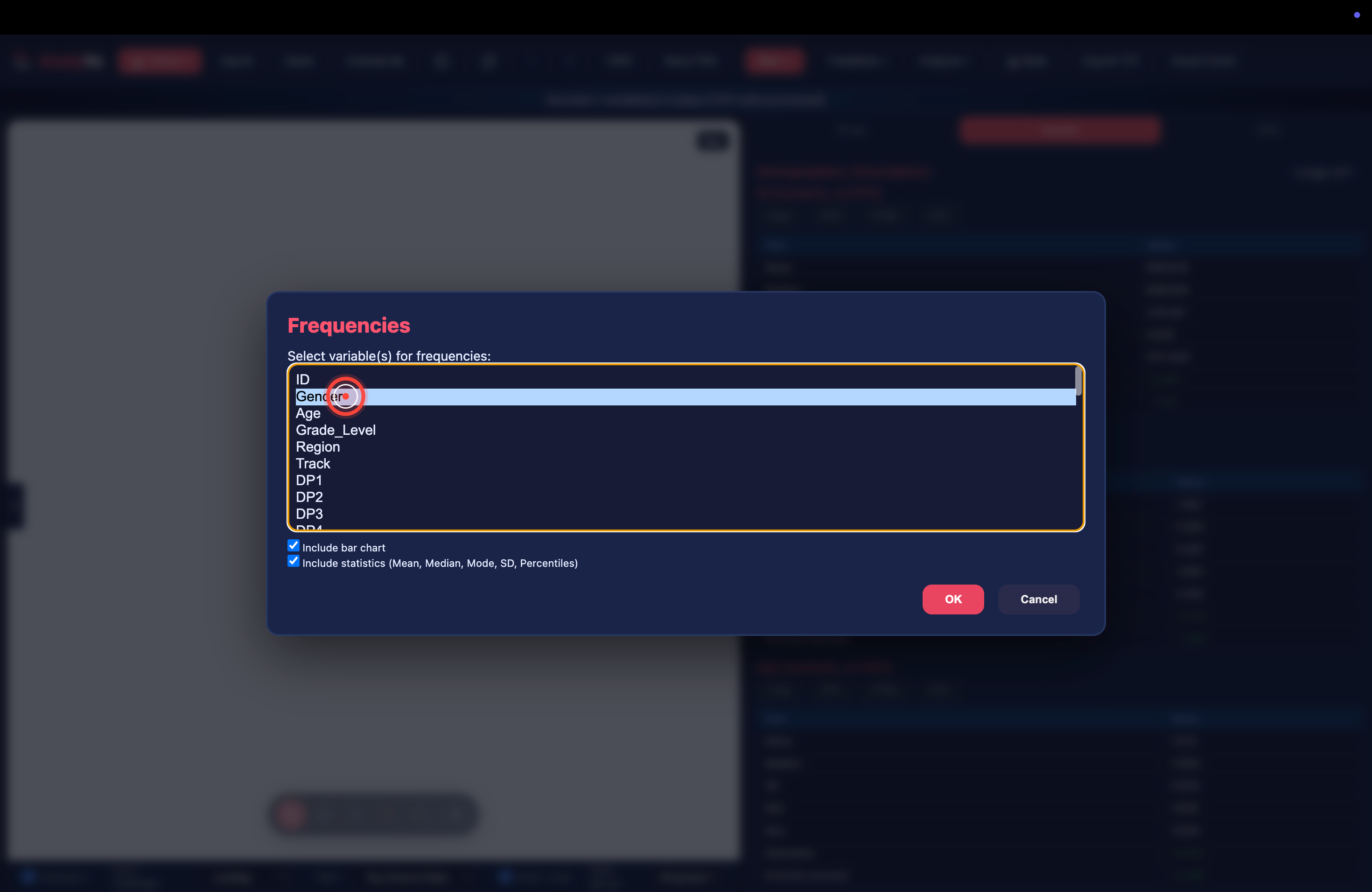
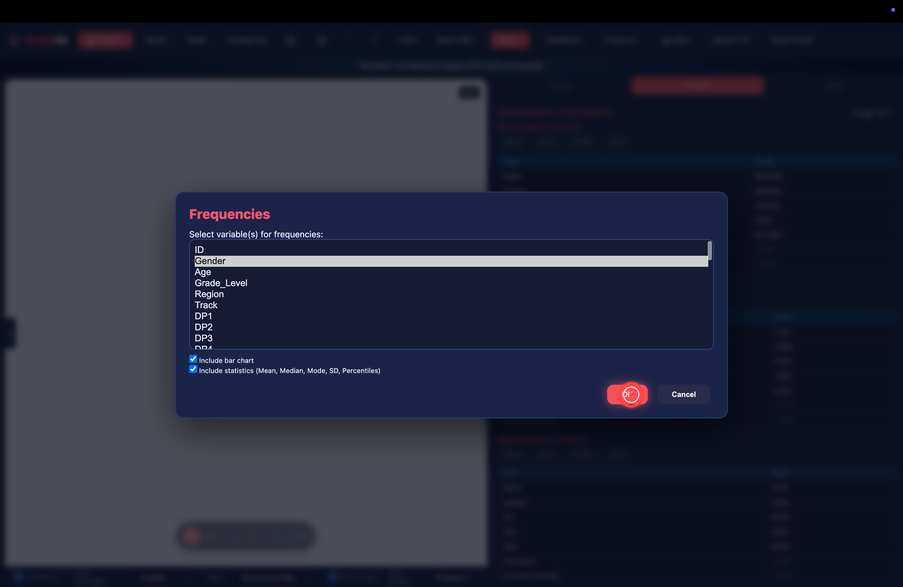
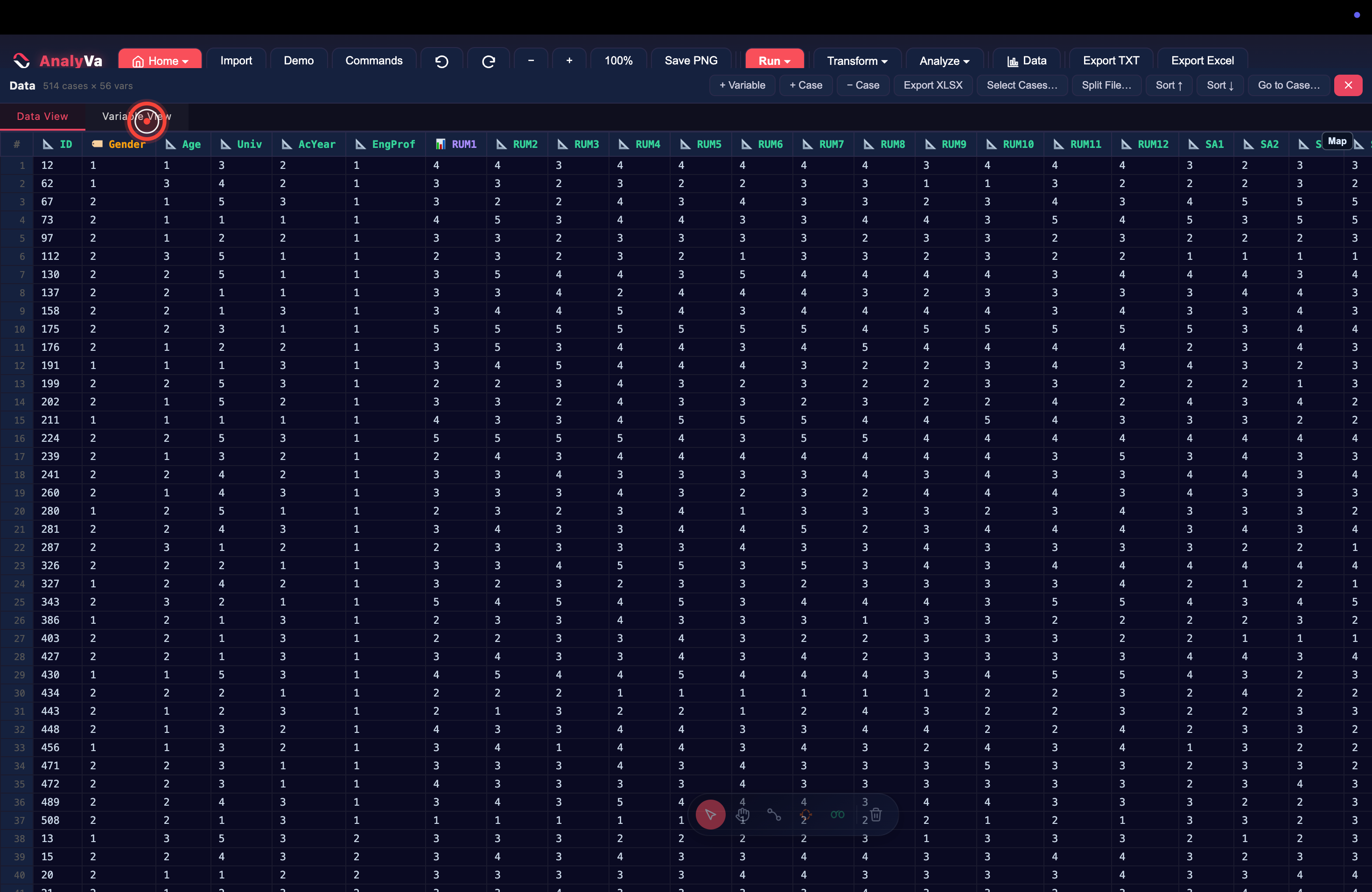
<p><strong>Step 7 — Select <em>Gender</em> and run.</strong>
Tick <strong>Include bar chart</strong> and <strong>Include statistics</strong> to get both a
distribution table and a visual.</p>

<p><img src="/blog/images/analyva-mga-07.png" alt="The Frequencies dialog with Gender selected and bar chart option checked" /></p>

<p><strong>Step 8 — Click <em>OK</em>.</strong></p>

<p><img src="/blog/images/analyva-mga-08.png" alt="The Frequencies dialog ready to run on Gender" /></p>

<p>The output confirms the recode worked: 55.2% one label, 44.8% the
other, labeled — not <code class="language-plaintext highlighter-rouge">1</code> and <code class="language-plaintext highlighter-rouge">2</code> — in every subsequent table.</p>

<h2 id="running-multi-group-analysis">Running multi-group analysis</h2>

<p>With a labeled grouping variable confirmed, the PLS-SEM dialog can
split the estimation by group. AnalyVa’s built-in <strong>TAM</strong> demo dataset
already ships with a two-construct model (<code class="language-plaintext highlighter-rouge">PU</code>, <code class="language-plaintext highlighter-rouge">PEOU</code>) and its own
<code class="language-plaintext highlighter-rouge">Gender</code> variable, which makes it a fast way to see the grouped-run
option end to end — the same <strong>Group data sets</strong> control works
identically on your own recoded variable.</p>

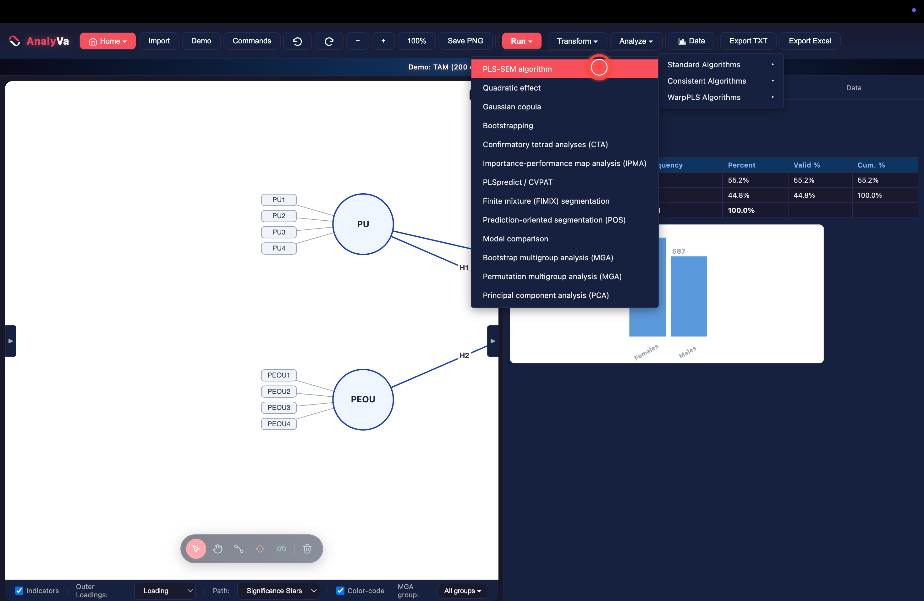
<p><strong>Step 9 — Open <em>Run → PLS-SEM</em> on a model with a grouping variable
available.</strong>
The full PLS-SEM submenu includes both <strong>Bootstrap multigroup analysis
(MGA)</strong> and <strong>Permutation multigroup analysis (MGA)</strong> as dedicated
significance tests for group differences — useful once the basic
grouped run below establishes there’s a difference worth testing.</p>

<p><img src="/blog/images/analyva-mga-09.png" alt="The Run &gt; PLS-SEM submenu showing Bootstrap MGA and Permutation MGA options" /></p>

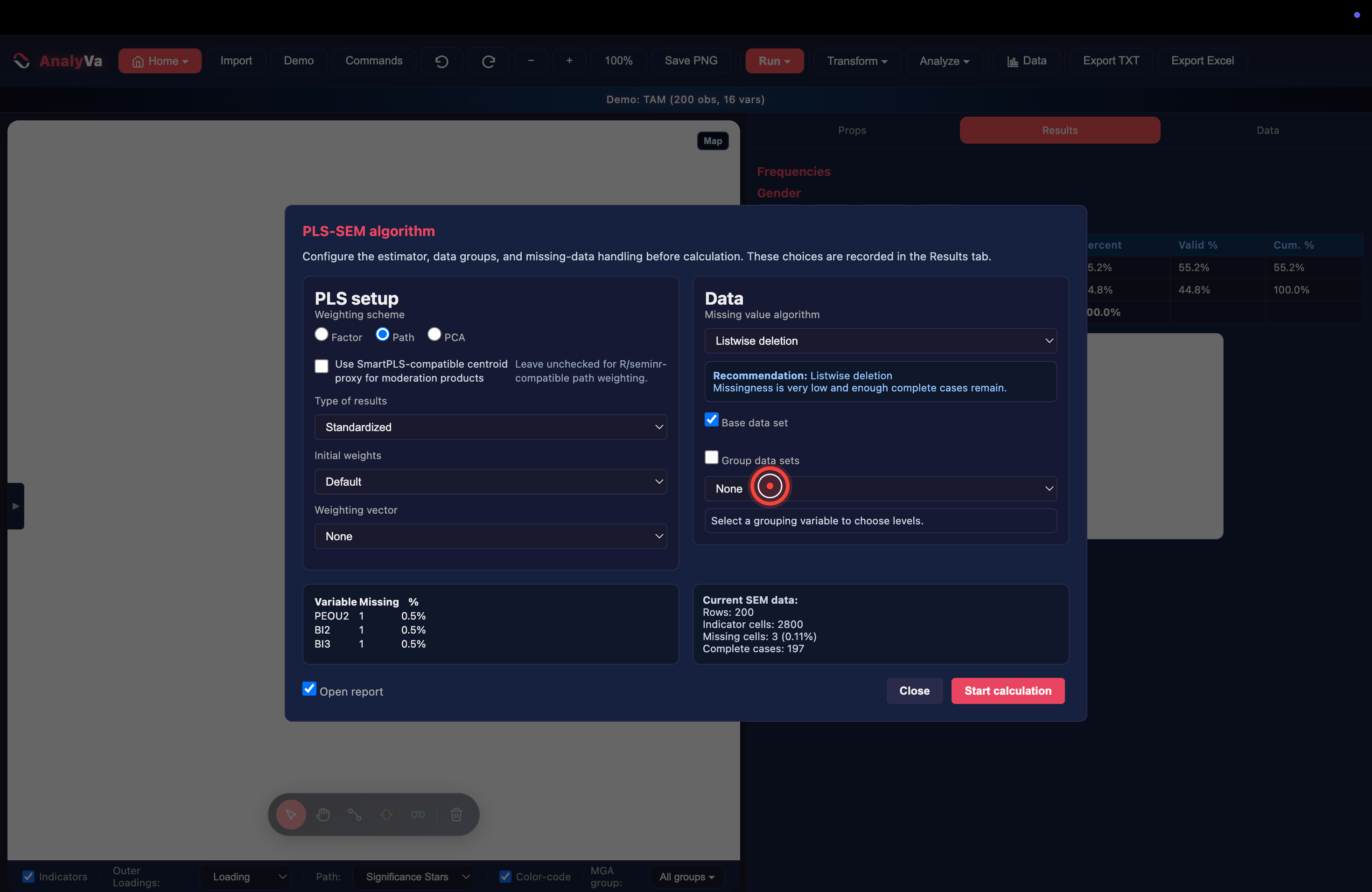
<p><strong>Step 10 — Open the PLS-SEM algorithm dialog.</strong>
By default, <strong>Group data sets</strong> is unchecked and the dropdown reads
<strong>None</strong> — the algorithm runs on the full sample.</p>

<p><img src="/blog/images/analyva-mga-10.png" alt="The PLS-SEM algorithm dialog with Group data sets unchecked" /></p>

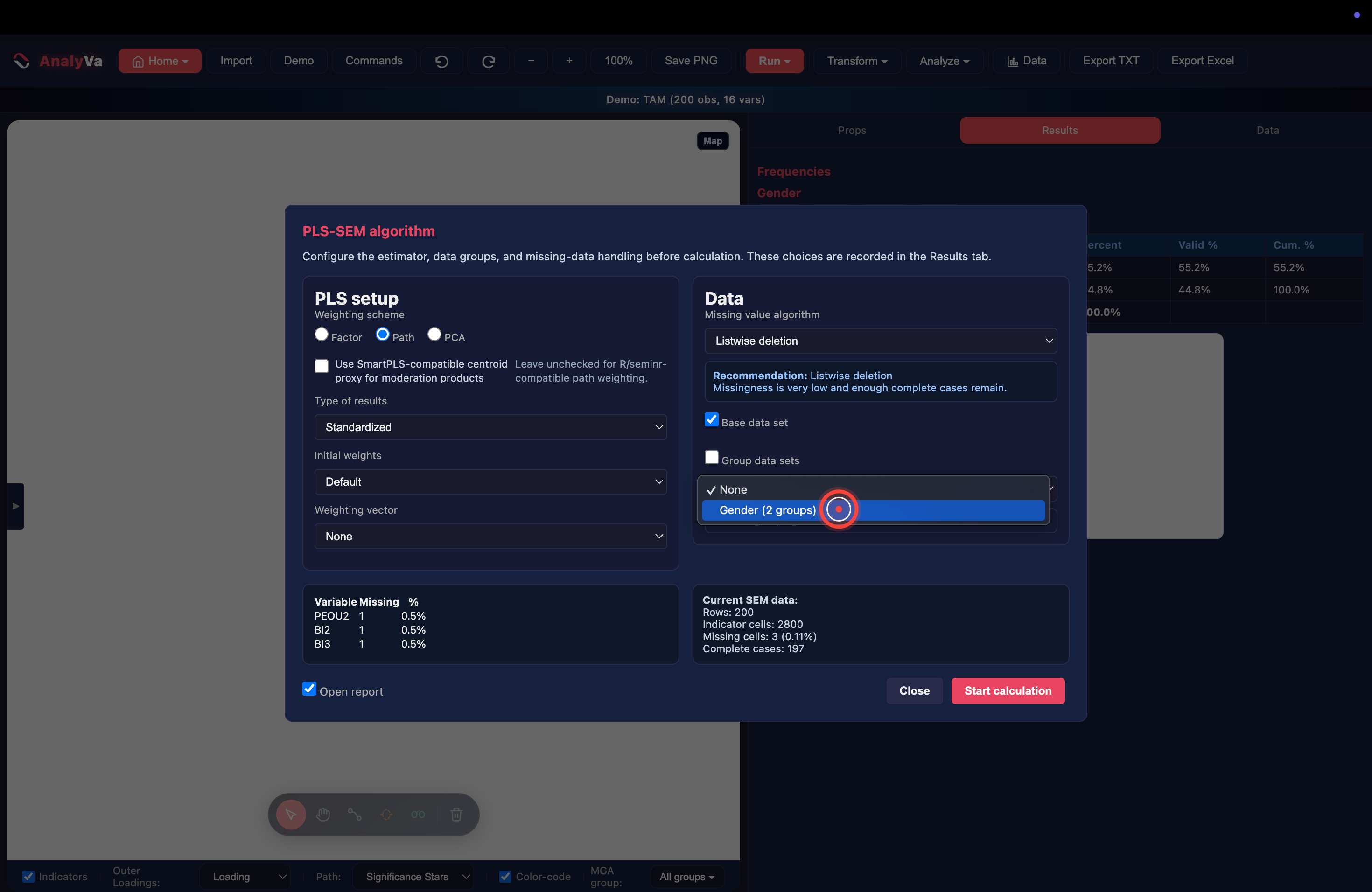
<p><strong>Step 11 — Tick <em>Group data sets</em> and pick the grouping variable.</strong>
Once checked, the dropdown lists every eligible categorical variable in
the dataset. Select <strong>Gender (2 groups)</strong>.</p>

<p><img src="/blog/images/analyva-mga-11.png" alt="The Group data sets dropdown open, Gender (2 groups) highlighted" /></p>

<p><strong>Step 12 — Confirm both levels and <em>Start calculation</em>.</strong>
Checkboxes for <strong>Female</strong> and <strong>Male</strong> appear, both ticked by default —
uncheck either to run a single-group subset instead of a full
comparison. Leave both checked and click <strong>Start calculation</strong>.</p>

<p><img src="/blog/images/analyva-mga-12.png" alt="Female and Male checkboxes both ticked, Start calculation highlighted" /></p>

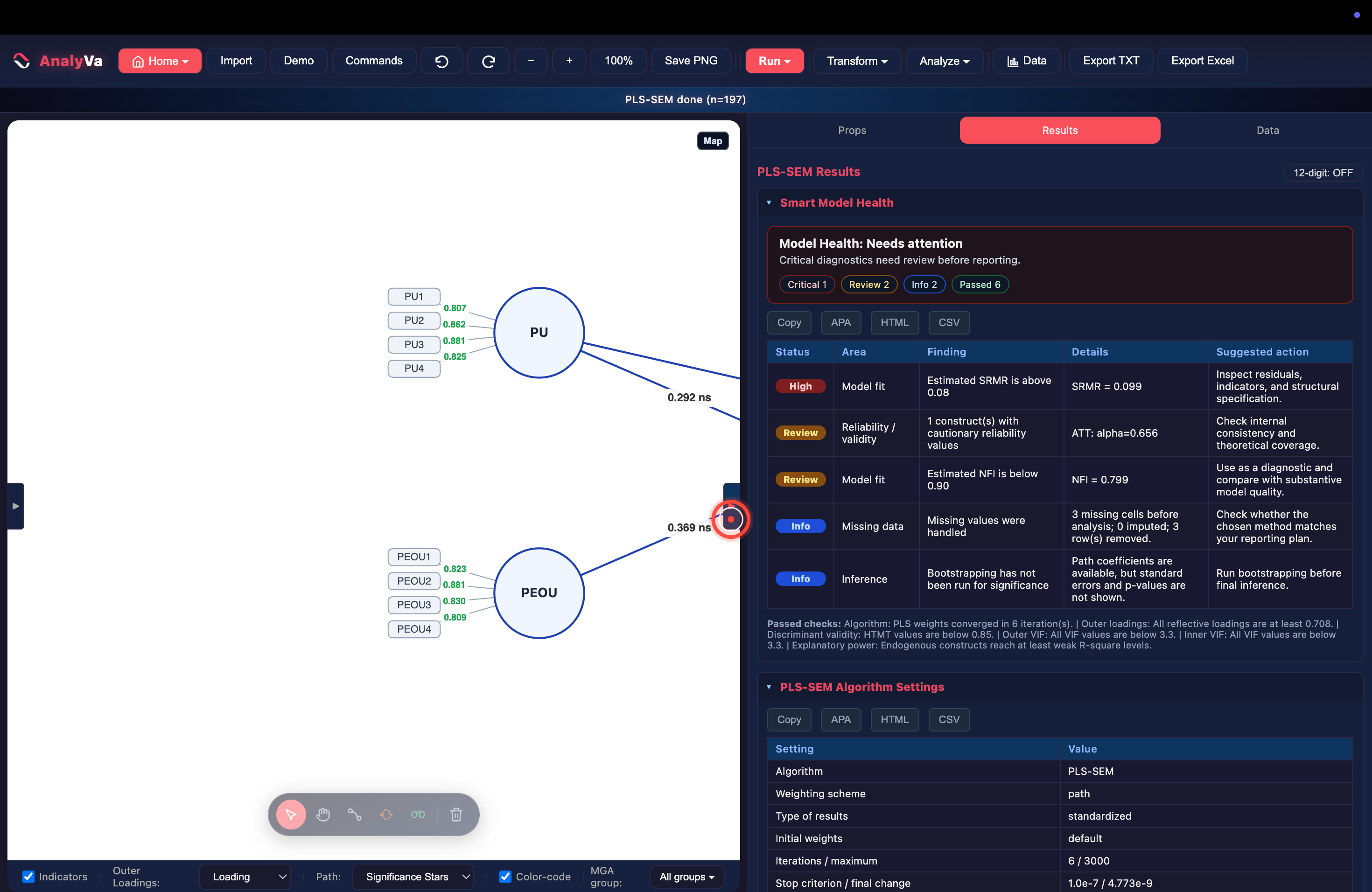
<p><strong>Step 13 — Read the result.</strong>
AnalyVa reports <em>“PLS-SEM done (n=197)”</em> — the complete-case count
after listwise deletion — and opens straight into the <strong>Smart Model
Health</strong> panel, which flags model fit and reliability issues before you
even look at group-specific coefficients. A group selector
(<strong>MGA group: All groups</strong>) at the bottom toolbar lets you flip the
canvas between the pooled model and each group’s own path diagram.</p>

<p><img src="/blog/images/analyva-mga-13.png" alt="The completed grouped run with the Smart Model Health panel and MGA group selector" /></p>

<h2 id="what-comes-next">What comes next</h2>

<p>A grouped PLS-SEM run gives you two sets of path coefficients side by
side, but eyeballing a difference between 0.32 and 0.41 isn’t a
significance test. That’s what <strong>Bootstrap MGA</strong> and <strong>Permutation
MGA</strong> — both visible in the Run menu above — are for: they resample
within each group and report whether the path difference survives
inference. Run the basic grouped estimation first to see whether a
difference is worth testing, then reach for one of the two MGA
procedures to confirm it statistically.</p>]]></content><author><name>Abdelouahd Bouzar</name><email>support@analyva.com</email></author><category term="PLS-SEM" /><category term="analyva" /><category term="pls-sem" /><category term="mga" /><category term="recoding" /><summary type="html"><![CDATA[Turn a numeric grouping variable into labeled categories with Recode into Same Variables, then enable Group data sets in the PLS-SEM dialog to run a two-group multi-group analysis.]]></summary><media:thumbnail xmlns:media="http://search.yahoo.com/mrss/" url="https://analyva.com/blog/images/cover-mga.svg" /><media:content medium="image" url="https://analyva.com/blog/images/cover-mga.svg" xmlns:media="http://search.yahoo.com/mrss/" /></entry><entry><title type="html">PLS-SEM in AnalyVa: Building a Model and Cleaning Weak Indicators</title><link href="https://analyva.com/blog/pls-sem-with-indicator-cleaning/" rel="alternate" type="text/html" title="PLS-SEM in AnalyVa: Building a Model and Cleaning Weak Indicators" /><published>2026-08-04T00:00:00+00:00</published><updated>2026-08-04T00:00:00+00:00</updated><id>https://analyva.com/blog/pls-sem-with-indicator-cleaning</id><content type="html" xml:base="https://analyva.com/blog/pls-sem-with-indicator-cleaning/"><![CDATA[<p>A PLS-SEM model rarely comes out clean on the first run. Somewhere in a
16-item construct there’s an indicator with a 0.68 loading that a
reviewer will flag, and finding it by scanning a results table is slow.
This post walks through building a four-construct model in AnalyVa,
running the algorithm, and using the loadings display — plus the
built-in model-health diagnostics — to find and drop the weak
indicators without leaving the canvas.</p>

<h2 id="importing-the-data">Importing the data</h2>

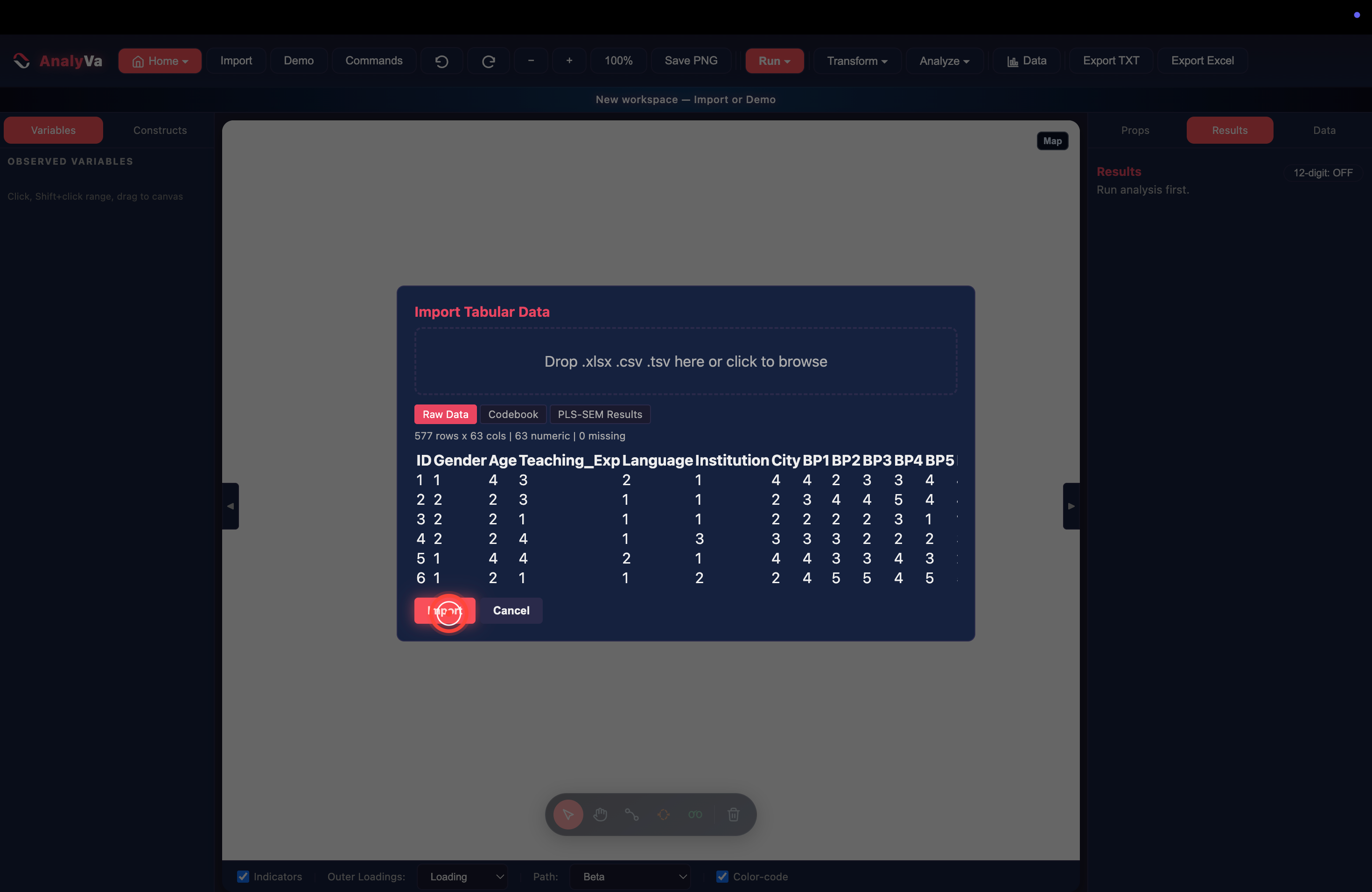
<p><strong>Step 1 — Click <em>Import</em>.</strong>
On a fresh workspace, the canvas is empty and the Results panel just
says <em>“Run analysis first.”</em> Click <strong>Import</strong> in the top toolbar.</p>

<p><img src="/blog/images/analyva-plssem-01.png" alt="The Import button highlighted on an empty AnalyVa canvas" /></p>

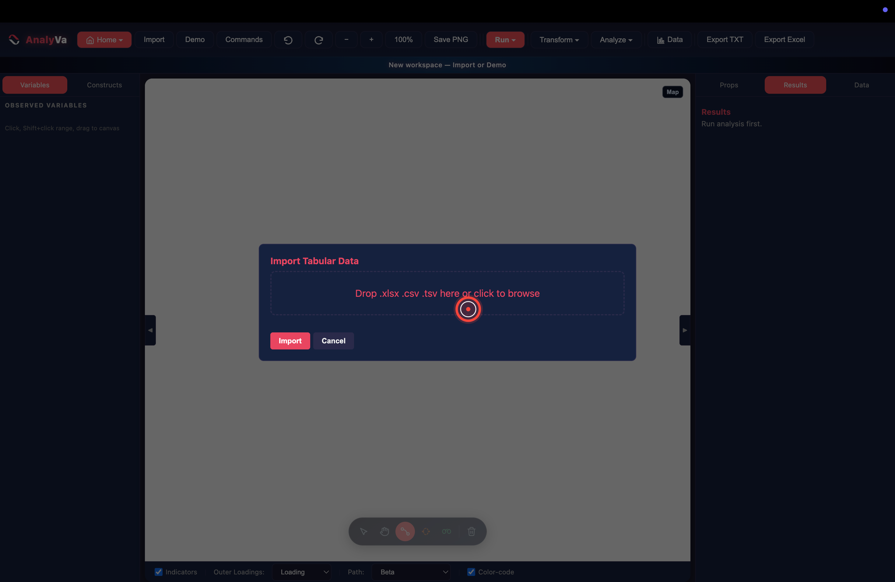
<p><strong>Step 2 — Drop the file.</strong>
The <strong>Import Tabular Data</strong> dialog accepts <code class="language-plaintext highlighter-rouge">.xlsx</code>, <code class="language-plaintext highlighter-rouge">.csv</code>, or <code class="language-plaintext highlighter-rouge">.tsv</code>.</p>

<p><img src="/blog/images/analyva-plssem-02.png" alt="The Import Tabular Data dialog waiting for a file" /></p>

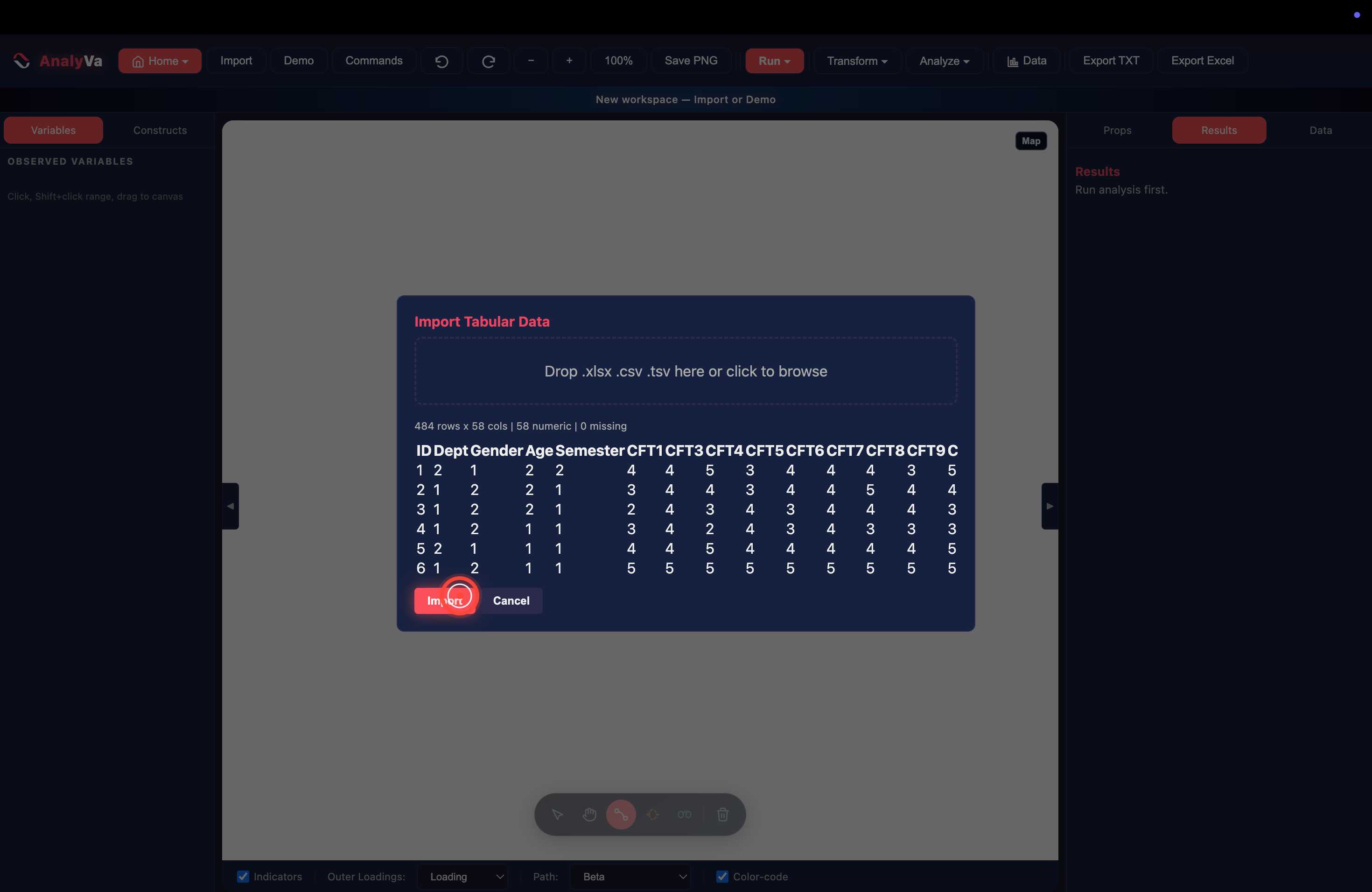
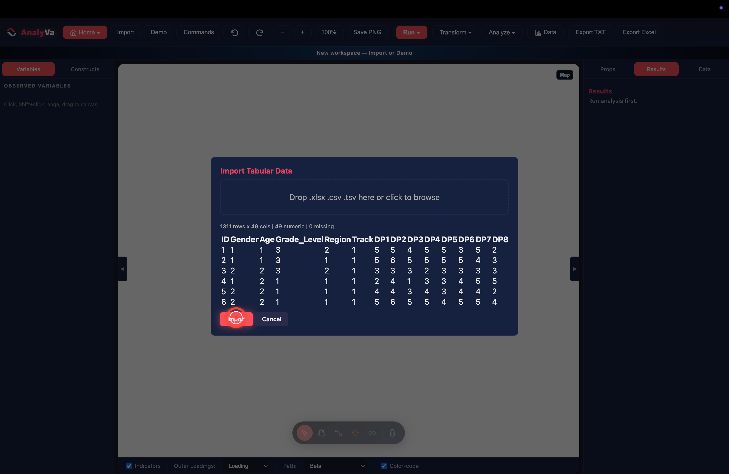
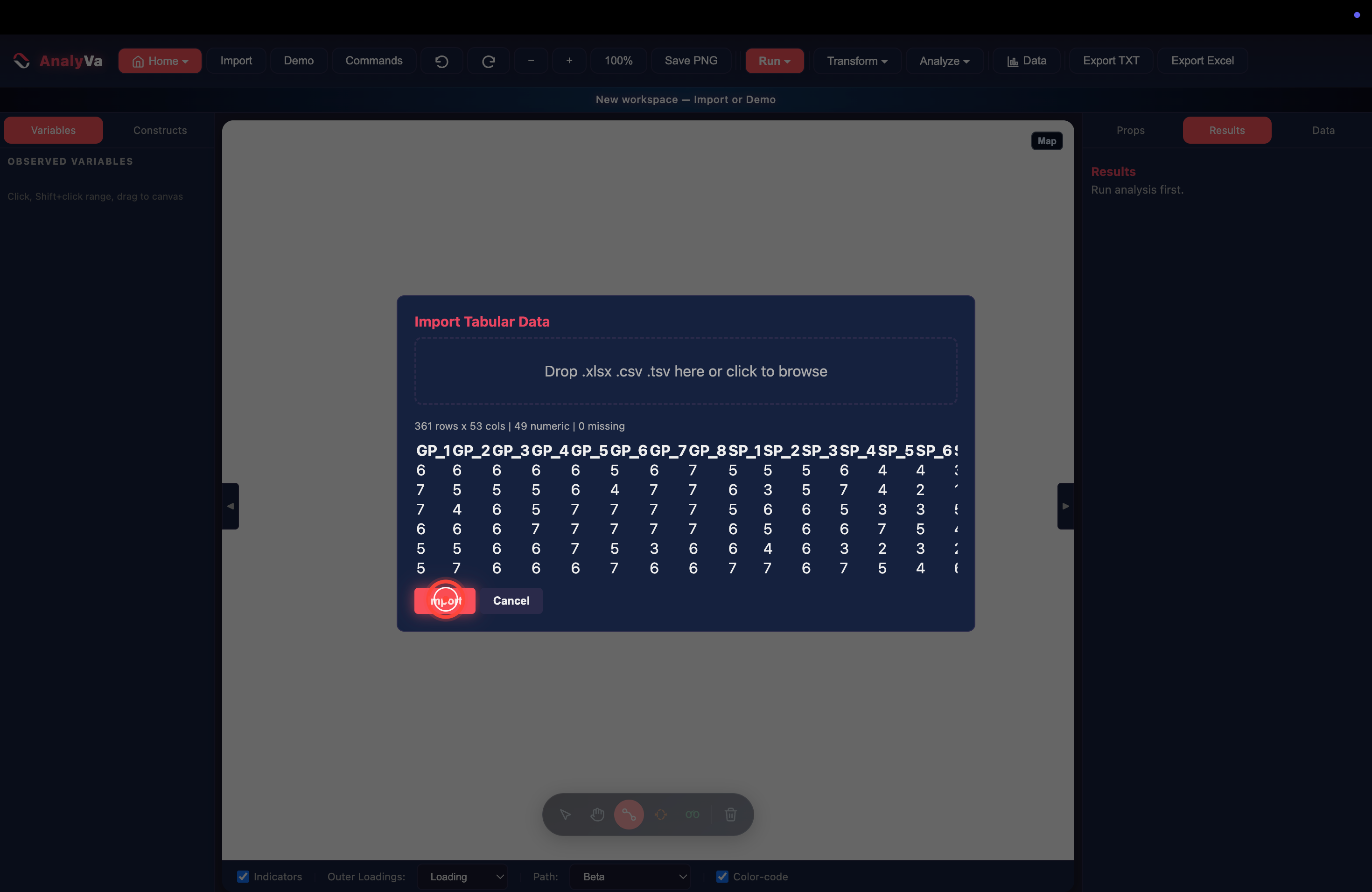
<p><strong>Step 3 — Check the preview and import.</strong>
AnalyVa parses the file and reports the shape before you commit — here,
484 rows × 58 columns, all numeric, no missing values. The first six
rows are shown for a sanity check. Click <strong>Import</strong>.</p>

<p><img src="/blog/images/analyva-plssem-03.png" alt="The import preview showing 484 rows by 58 columns" /></p>

<h2 id="building-a-four-construct-model">Building a four-construct model</h2>

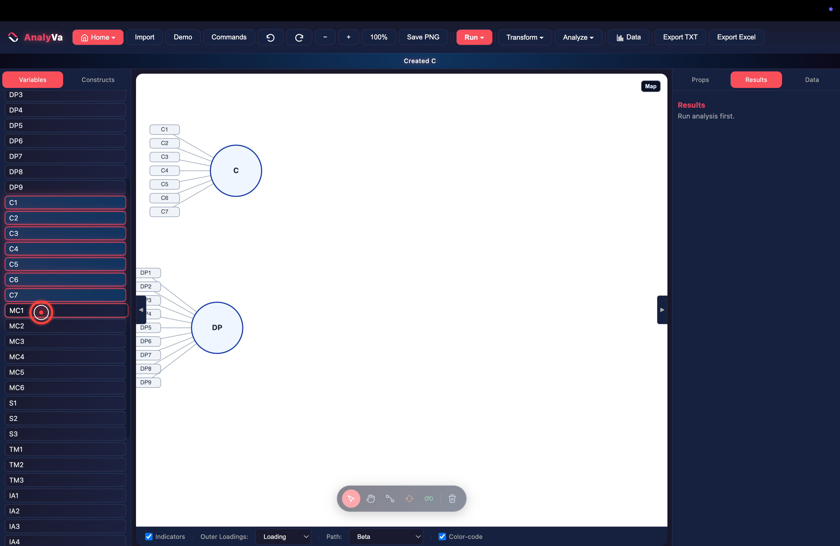
<p>The dataset holds four independent constructs — <strong>CFT</strong>, <strong>PFT</strong>,
<strong>WM</strong>, and <strong>WA</strong> — all predicting a single outcome, <strong>WSE</strong>. Building
each construct is the same click-shift-click-drag pattern used
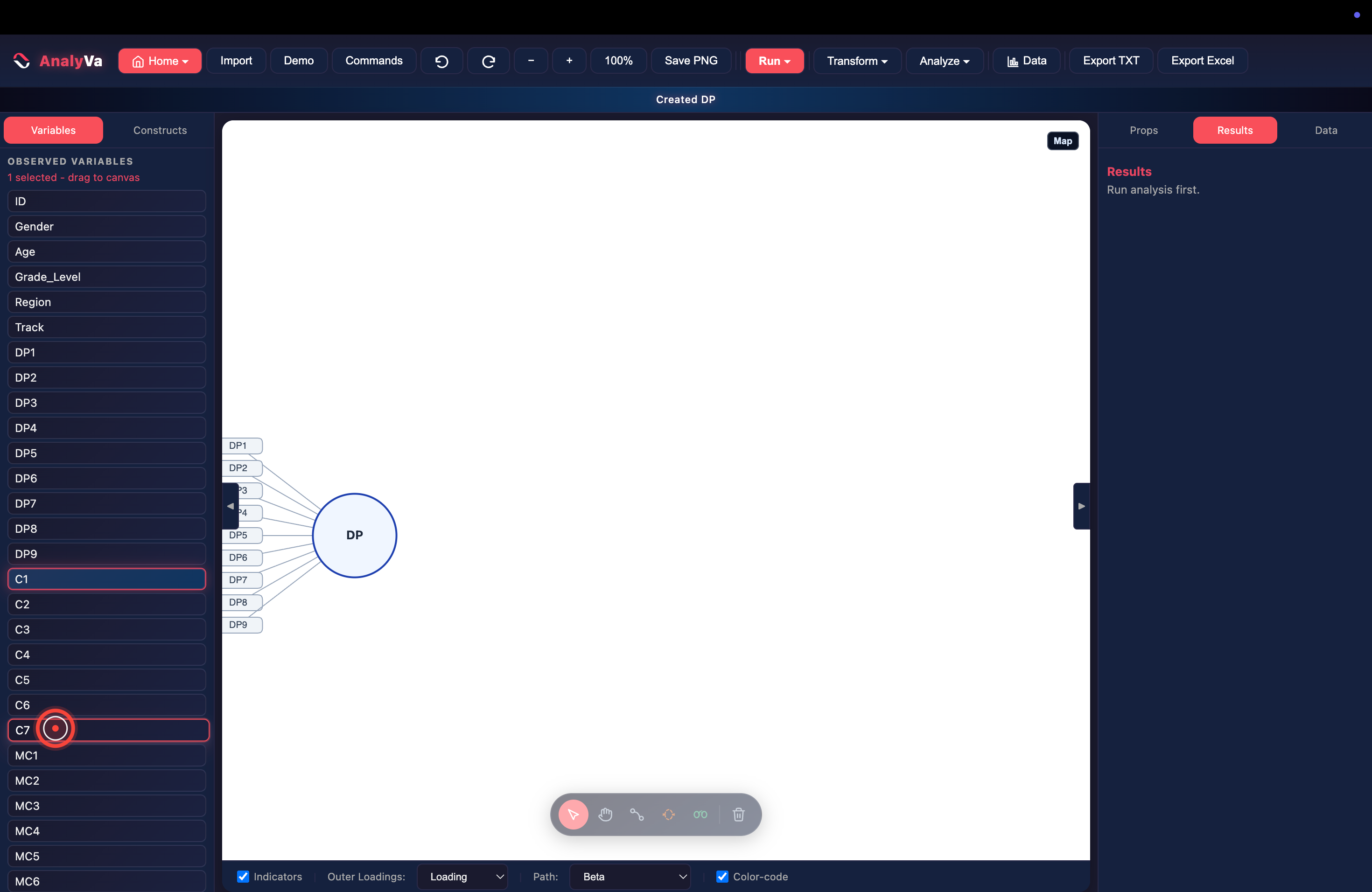
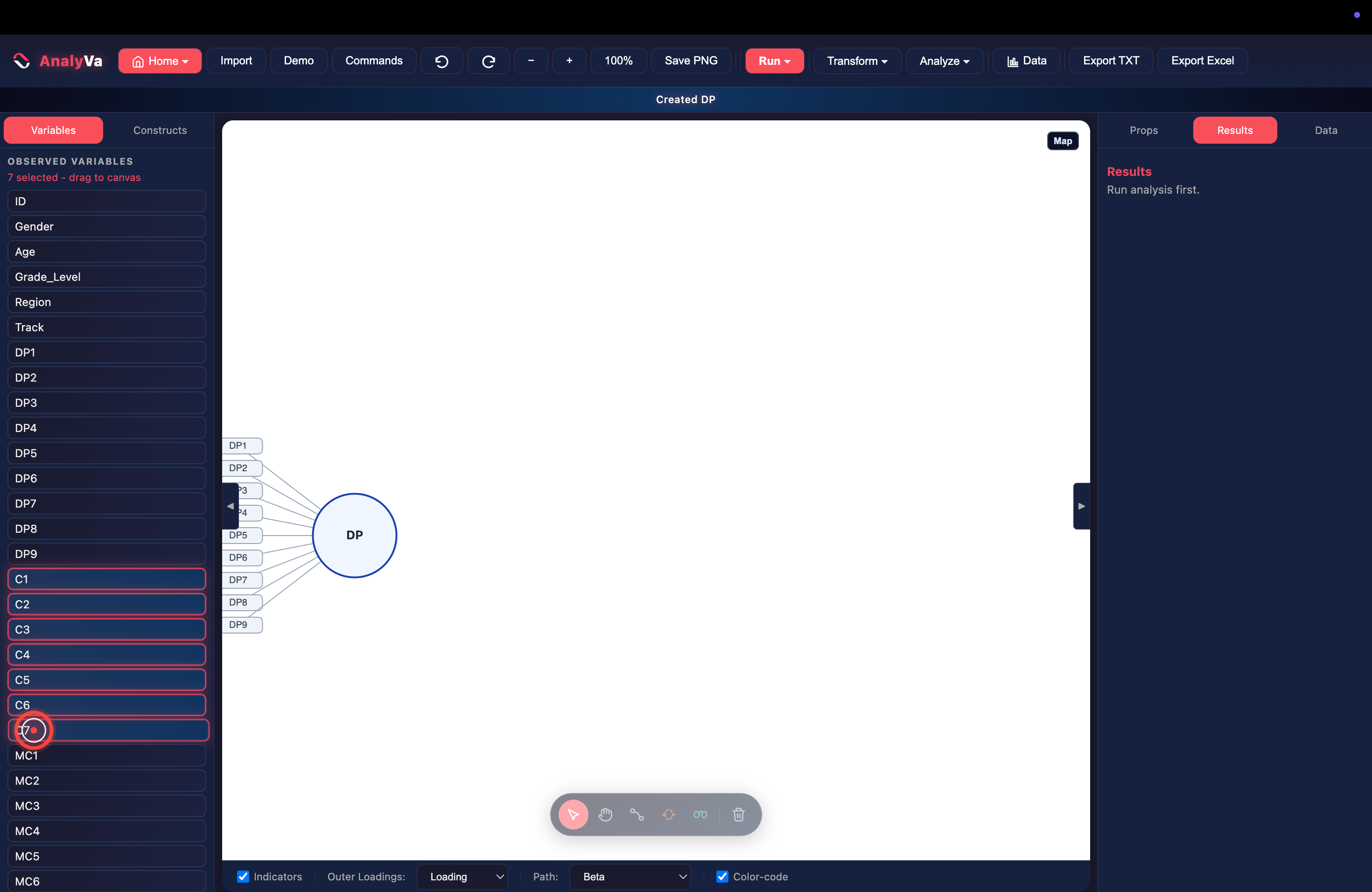
throughout AnalyVa: click an indicator’s first item in the sidebar,
shift-click the last, and drag the highlighted range onto the canvas.
Repeat for each block, then switch to the Path tool and draw a
connection between every predictor and WSE.</p>

<p><strong>Step 4 — The full model with all eight hypothesis paths.</strong>
CFT and PFT each predict WM and WA directly, and all four predict WSE —
eight paths in total (H1–H8). Clicking the WSE construct switches the
right panel to <strong>Props</strong>, listing all 9 of its indicators along with
<strong>Delete Selected</strong>, <strong>Select All</strong>, and <strong>Clear</strong> buttons — the same
controls used later for indicator cleanup.</p>

<p><img src="/blog/images/analyva-plssem-04.png" alt="The full four-construct model with H1 through H8 drawn, Run menu open on PLS-SEM" /></p>

<h2 id="running-the-algorithm">Running the algorithm</h2>

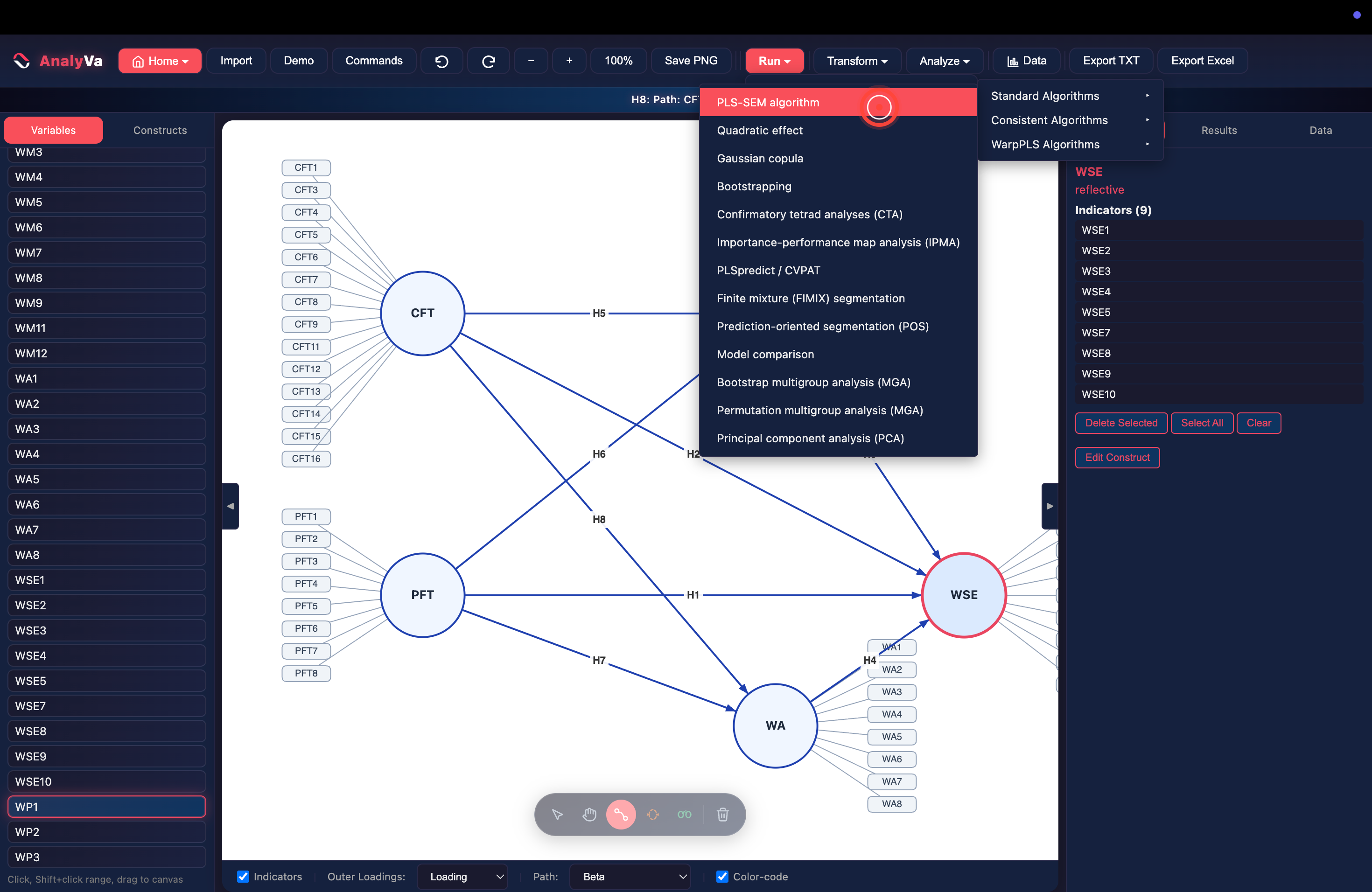
<p><strong>Step 5 — Open <em>Run → PLS-SEM → Standard Algorithms → PLS-SEM
algorithm</em>.</strong></p>

<p><img src="/blog/images/analyva-plssem-05.png" alt="The PLS-SEM submenu with Standard Algorithms expanded" /></p>

<p><strong>Step 6 — Configure and click <em>Start calculation</em>.</strong>
The configuration dialog defaults to the Hair et al. recommendations:
<strong>Path</strong> weighting scheme, <strong>Standardized</strong> results, <strong>Mean
replacement</strong> for missing values (moot here — AnalyVa confirms zero
missing cells across the 484 rows). Leave the defaults and click
<strong>Start calculation</strong>.</p>

<p><img src="/blog/images/analyva-plssem-06.png" alt="The PLS-SEM algorithm configuration dialog with Start calculation highlighted" /></p>

<h2 id="reading-the-smart-model-health-panel">Reading the Smart Model Health panel</h2>

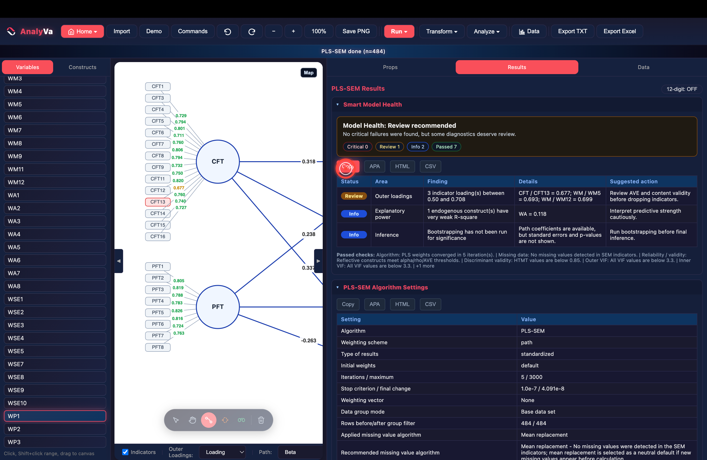
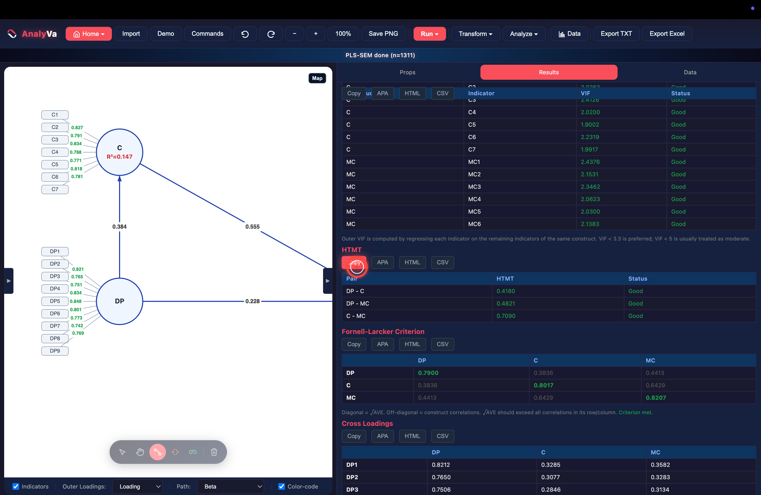
<p><strong>Step 7 — Check the diagnostics before touching the loadings.</strong>
The Results tab opens with a <strong>Smart Model Health</strong> summary before any
other output. For this run it reads <em>“Review recommended”</em> — no
critical failures, but the checklist flags something specific:</p>

<blockquote>
  <p><strong>Review — Outer loadings.</strong> 3 indicator loading(s) between 0.50 and
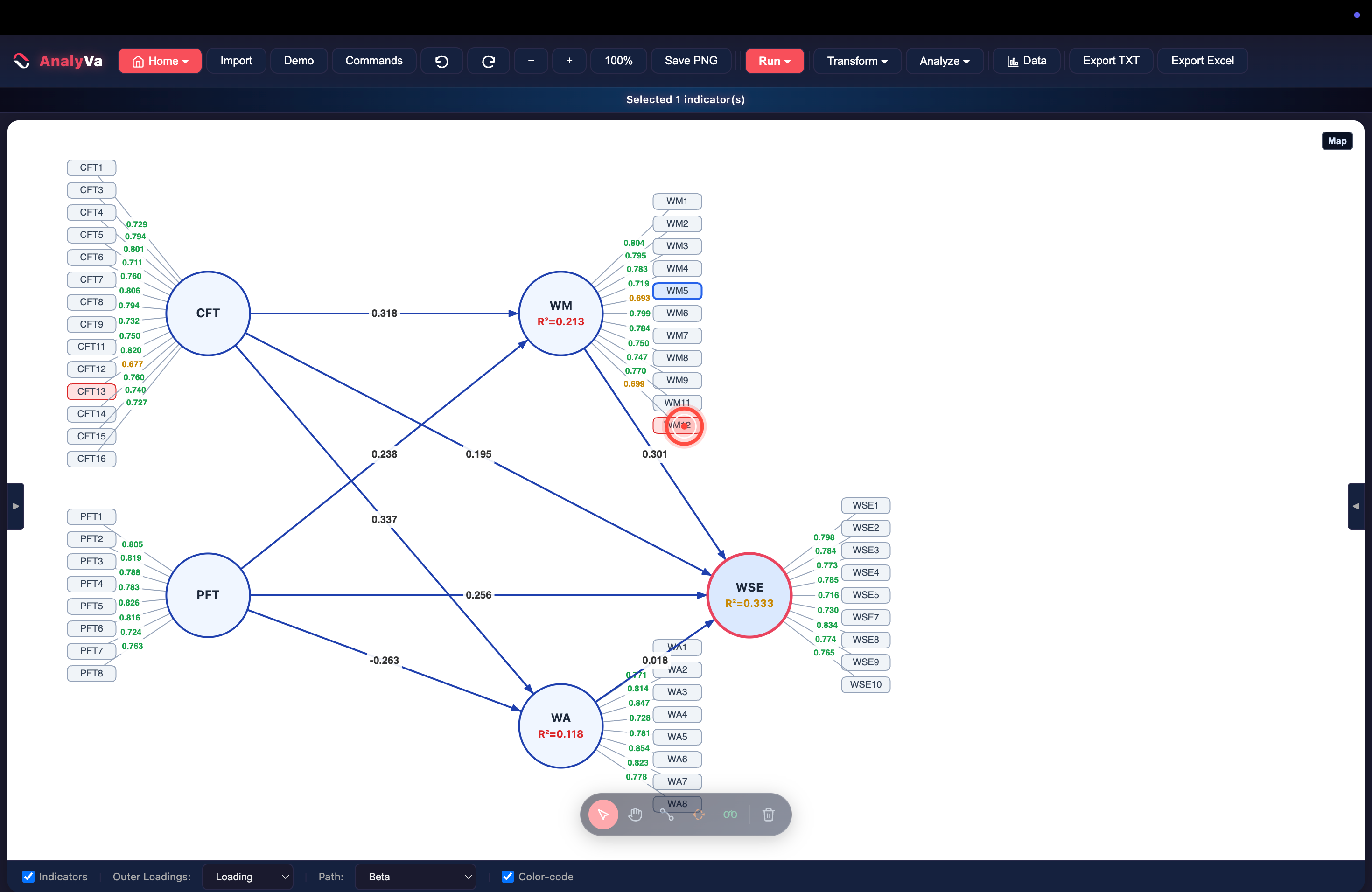
0.708: <code class="language-plaintext highlighter-rouge">CFT / CFT13 = 0.677</code>; <code class="language-plaintext highlighter-rouge">WM / WM5 = 0.693</code>; <code class="language-plaintext highlighter-rouge">WM / WM12 = 0.699</code>.
<em>Suggested action: review AVE and content validity before dropping
indicators.</em></p>
</blockquote>

<p>That one line does the scanning work for you — no need to hunt through
a loadings table for the offenders. AnalyVa also flags that WA’s
R² (0.118) is weak and that bootstrapping hasn’t been run yet, both
worth remembering for later.</p>

<p><img src="/blog/images/analyva-plssem-07.png" alt="The Smart Model Health panel listing three weak outer loadings by name" /></p>

<p><strong>Step 8 — Find the same indicators on the canvas.</strong>
With <strong>Color-code</strong> enabled at the bottom toolbar, loadings below the
0.708 rule-of-thumb render in amber instead of green — the same three
values the health panel already named. <code class="language-plaintext highlighter-rouge">WM12</code> is selected here (its
loading, 0.699, sits right on the canvas next to it) and <code class="language-plaintext highlighter-rouge">CFT13</code> is
outlined in red.</p>

<p><img src="/blog/images/analyva-plssem-08.png" alt="The canvas with WM12 selected and its 0.699 loading shown in amber, CFT13 outlined in red" /></p>

<h2 id="dropping-the-weak-indicators">Dropping the weak indicators</h2>

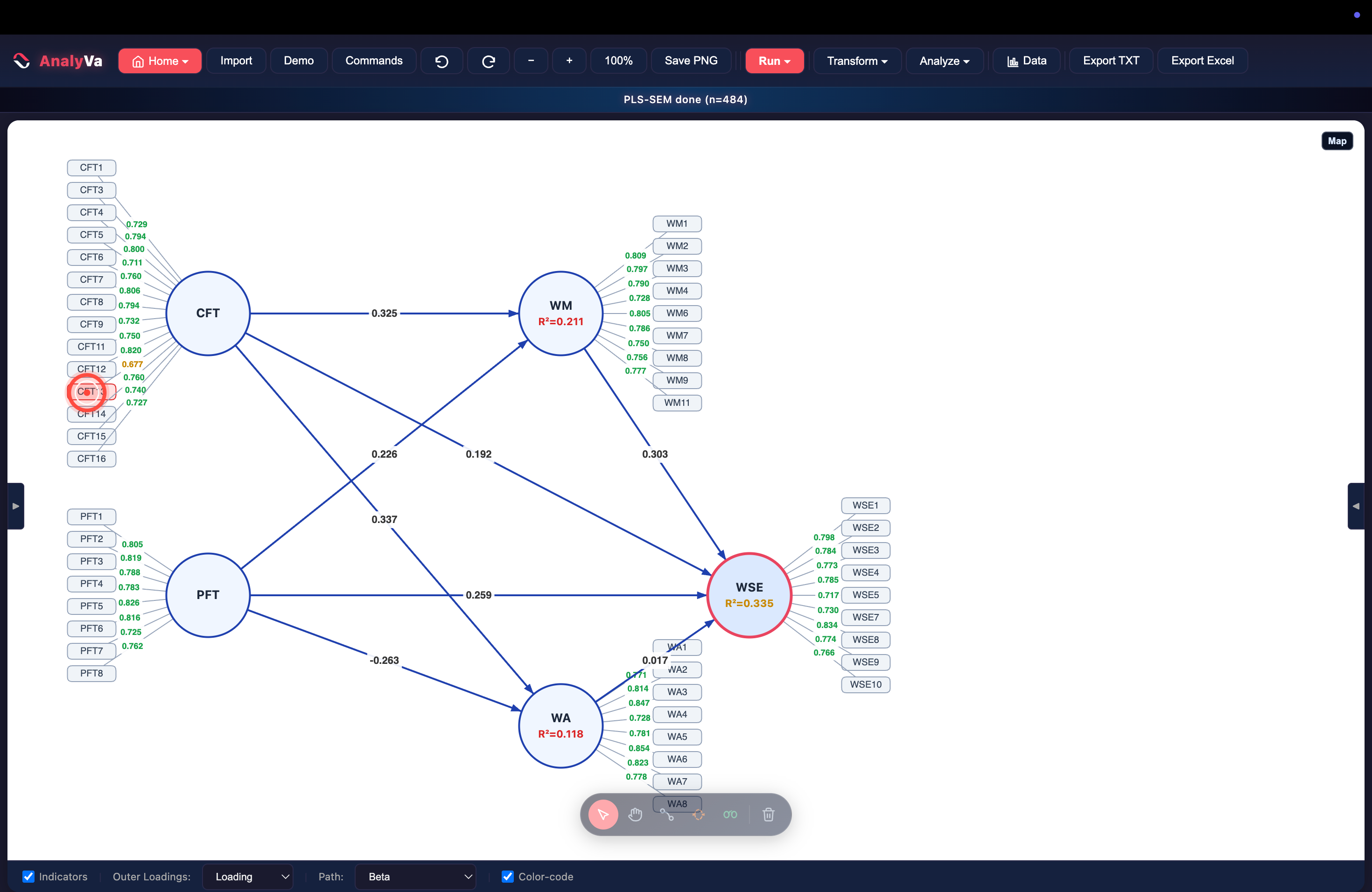
<p><strong>Step 9 — Select the offending indicator in the sidebar.</strong>
Click <code class="language-plaintext highlighter-rouge">CFT13</code> in the left sidebar (or on the canvas). It highlights in
red to confirm the selection.</p>

<p><img src="/blog/images/analyva-plssem-09.png" alt="CFT13 highlighted in red in the sidebar, ready to delete" /></p>

<p>Select the construct on the canvas, switch to its <strong>Props</strong> panel, tick
the indicator(s) to remove — <code class="language-plaintext highlighter-rouge">CFT13</code> and <code class="language-plaintext highlighter-rouge">WM12</code> — and click <strong>Delete
Selected</strong>. AnalyVa updates the construct’s indicator list immediately;
no separate confirmation step.</p>

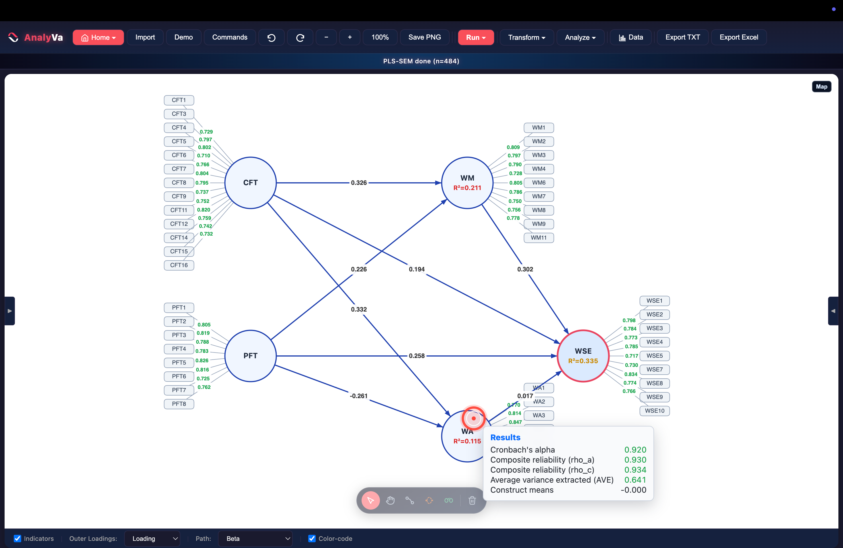
<p><strong>Step 10 — Re-run and check reliability.</strong>
With the weak indicators gone, re-run <em>PLS-SEM algorithm</em> the same way
as Step 6. AnalyVa reports the run as <em>“PLS-SEM done (n=484)”</em>.
Hovering a construct now surfaces its reliability block directly on
the canvas:</p>

<ul>
  <li><strong>Cronbach’s alpha:</strong> 0.920</li>
  <li><strong>Composite reliability (rho_a):</strong> 0.930</li>
  <li><strong>Composite reliability (rho_c):</strong> 0.934</li>
  <li><strong>Average variance extracted (AVE):</strong> 0.641</li>
</ul>

<p>All comfortably above the 0.70 / 0.50 thresholds.</p>

<p><img src="/blog/images/analyva-plssem-10.png" alt="The re-run model with a reliability tooltip showing alpha 0.920 and AVE 0.641" /></p>

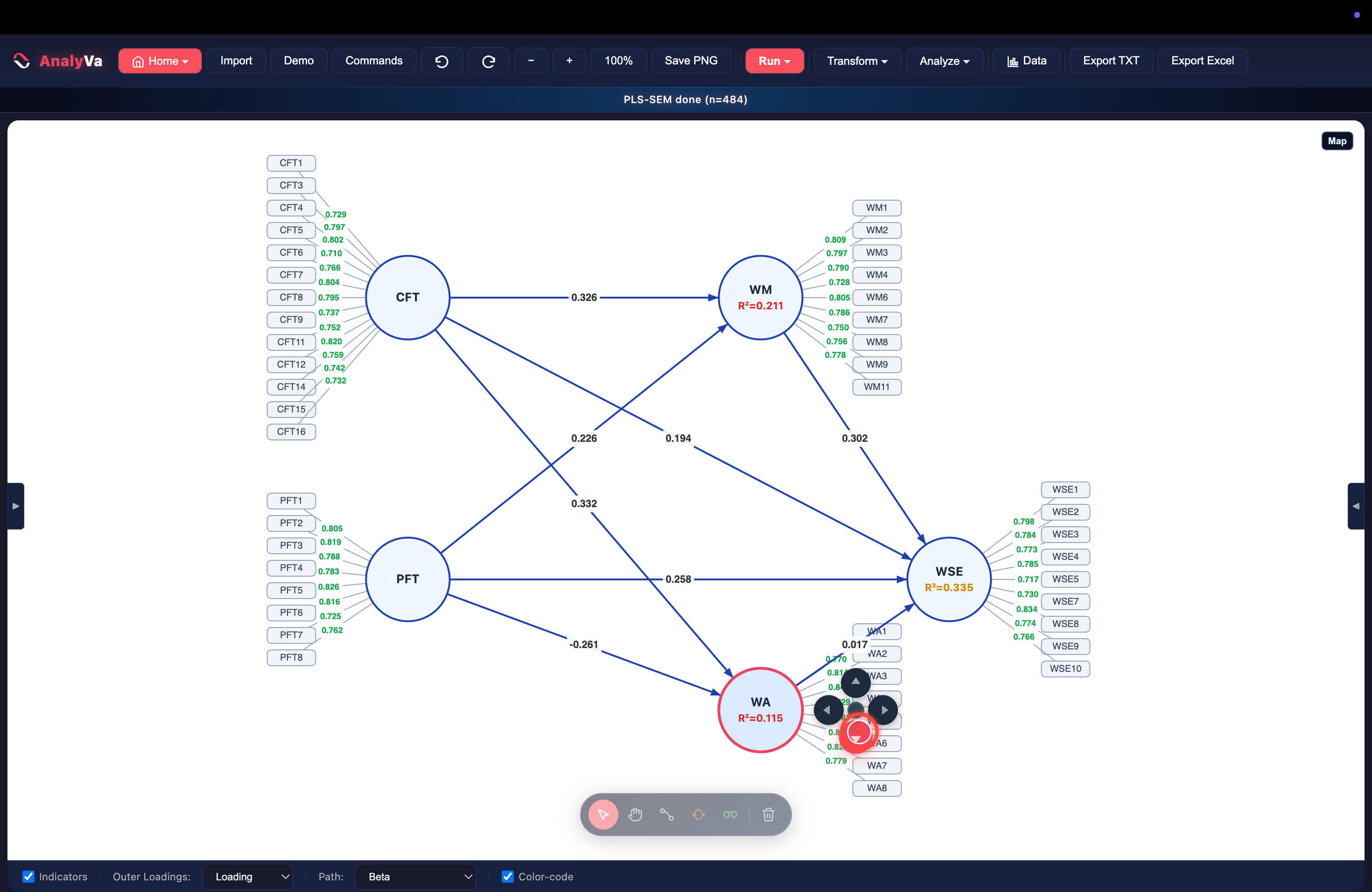
<p><strong>Step 11 — Confirm every remaining loading is clean.</strong>
<code class="language-plaintext highlighter-rouge">CFT</code> now runs <code class="language-plaintext highlighter-rouge">CFT1</code> through <code class="language-plaintext highlighter-rouge">CFT16</code> minus <code class="language-plaintext highlighter-rouge">CFT13</code>; <code class="language-plaintext highlighter-rouge">WM</code> runs <code class="language-plaintext highlighter-rouge">WM1</code>
through <code class="language-plaintext highlighter-rouge">WM11</code> minus <code class="language-plaintext highlighter-rouge">WM12</code>. Every visible loading is green.</p>

<p><img src="/blog/images/analyva-plssem-11.png" alt="The cleaned model with WM and CFT indicator lists updated" /></p>

<p><strong>Step 12 — The final model.</strong>
R² values barely move (WM: 0.211, WA: 0.115, WSE: 0.335 — practically
identical to the 12-indicator version), which is expected: two weak
formative-adjacent items rarely carry much of a reflective construct’s
explanatory power. What changes is defensibility — every loading in
the measurement model now clears 0.708 without an asterisk in the
write-up.</p>

<p><img src="/blog/images/analyva-plssem-12.png" alt="The final clean four-construct model with all outer loadings above 0.708" /></p>

<h2 id="why-this-matters-for-reporting">Why this matters for reporting</h2>

<p>Dropping indicators purely to inflate loadings is a real methodological
risk — reviewers know the difference between principled cleanup and
p-hacking a measurement model. The rule that keeps this defensible:
drop an indicator only when its loading is weak <em>and</em> the construct’s
AVE improves <em>and</em> the theoretical content coverage doesn’t collapse.
AnalyVa’s Smart Model Health panel gives you the first signal
automatically; the AVE and content-validity call is still yours to
make.</p>

<h2 id="the-order-that-matters">The order that matters</h2>

<ol>
  <li><strong>Build and run</strong> the full model first — don’t pre-emptively drop
indicators before seeing real loadings.</li>
  <li><strong>Read the Smart Model Health panel</strong> before scanning tables by eye.</li>
  <li><strong>Cross-check</strong> the flagged indicators against theoretical coverage,
not just the number.</li>
  <li><strong>Delete, re-run, and re-check</strong> reliability and AVE — never assume
removing one weak item won’t shift another.</li>
  <li><strong>Run bootstrapping</strong> before finalizing path significance (the
health panel will remind you if you forget).</li>
</ol>]]></content><author><name>Abdelouahd Bouzar</name><email>support@analyva.com</email></author><category term="PLS-SEM" /><category term="analyva" /><category term="pls-sem" /><category term="outer loadings" /><summary type="html"><![CDATA[Build a four-construct PLS-SEM model in AnalyVa, run the algorithm, and use the color-coded outer loadings to catch and remove indicators that are dragging down your measurement model.]]></summary><media:thumbnail xmlns:media="http://search.yahoo.com/mrss/" url="https://analyva.com/blog/images/cover-pls-cleaning.svg" /><media:content medium="image" url="https://analyva.com/blog/images/cover-pls-cleaning.svg" xmlns:media="http://search.yahoo.com/mrss/" /></entry><entry><title type="html">Qualitative Coding in AnalyVa: From Text Import to Coded Corpus</title><link href="https://analyva.com/blog/qualitative-coding-in-analyva/" rel="alternate" type="text/html" title="Qualitative Coding in AnalyVa: From Text Import to Coded Corpus" /><published>2026-08-02T00:00:00+00:00</published><updated>2026-08-02T00:00:00+00:00</updated><id>https://analyva.com/blog/qualitative-coding-in-analyva</id><content type="html" xml:base="https://analyva.com/blog/qualitative-coding-in-analyva/"><![CDATA[<p>Quantitative and qualitative analysis are usually taught in separate
courses, with separate software. AnalyVa combines both in one app —
switch workspaces once, and you have a full <strong>NVivo-style</strong> qualitative
coding environment with your familiar variables still available in the
other panel.</p>

<p>This post is the beginner’s tour of that workspace: from opening it
for the first time to a fully coded corpus you can query.</p>

<h2 id="opening-the-textual-analysis-workspace">Opening the Textual Analysis workspace</h2>

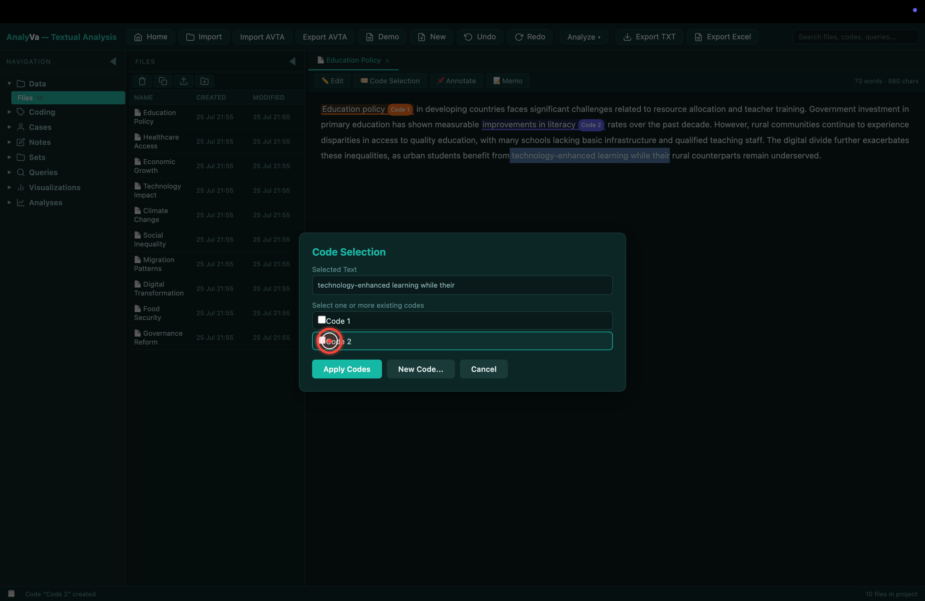
<p><strong>Step 1 — Pick <em>Textual Analysis</em> from the home screen.</strong>
When AnalyVa opens, you get two workspace cards: <strong>SEM &amp; Statistics</strong>
(the familiar quantitative side) and <strong>Textual Analysis</strong> (the
qualitative side). Click <strong>Launch Workspace</strong> on the second card.</p>

<p><img src="/blog/images/analyva-coding-01.png" alt="Home screen with Textual Analysis workspace ready to launch" /></p>

<p><strong>Step 2 — The Textual Analysis workspace loads.</strong>
The layout is three columns: a <strong>Navigation</strong> sidebar (Data, Coding,
Cases, Notes, Sets, Queries, Visualizations, Analyses), a <strong>Files</strong>
list in the middle, and a large document viewer on the right.</p>

<p><img src="/blog/images/analyva-coding-02.png" alt="Textual Analysis workspace loaded, ready to import files" /></p>

<h2 id="loading-a-corpus">Loading a corpus</h2>

<p><strong>Step 3 — Import your documents.</strong>
Click <strong>Import</strong> in the top toolbar and select <code class="language-plaintext highlighter-rouge">.txt</code>, <code class="language-plaintext highlighter-rouge">.pdf</code>,
<code class="language-plaintext highlighter-rouge">.docx</code>, or <code class="language-plaintext highlighter-rouge">.xlsx</code> files. Or, for a first walkthrough, click <strong>Demo</strong>
— AnalyVa ships with a set of 10 policy research documents you can
practice on without needing your own corpus first.</p>

<p><img src="/blog/images/analyva-coding-03.png" alt="Import options and the Demo shortcut in the toolbar" /></p>

<p><strong>Step 4 — Files appear in the Files list.</strong>
Each imported document becomes a row in the Files list with a created
and modified timestamp. In the demo corpus you get ten documents on
policy themes: Education Policy, Healthcare Access, Economic Growth,
Climate Change, and so on.</p>

<p><img src="/blog/images/analyva-coding-04.png" alt="The demo corpus loaded, 10 documents listed" /></p>

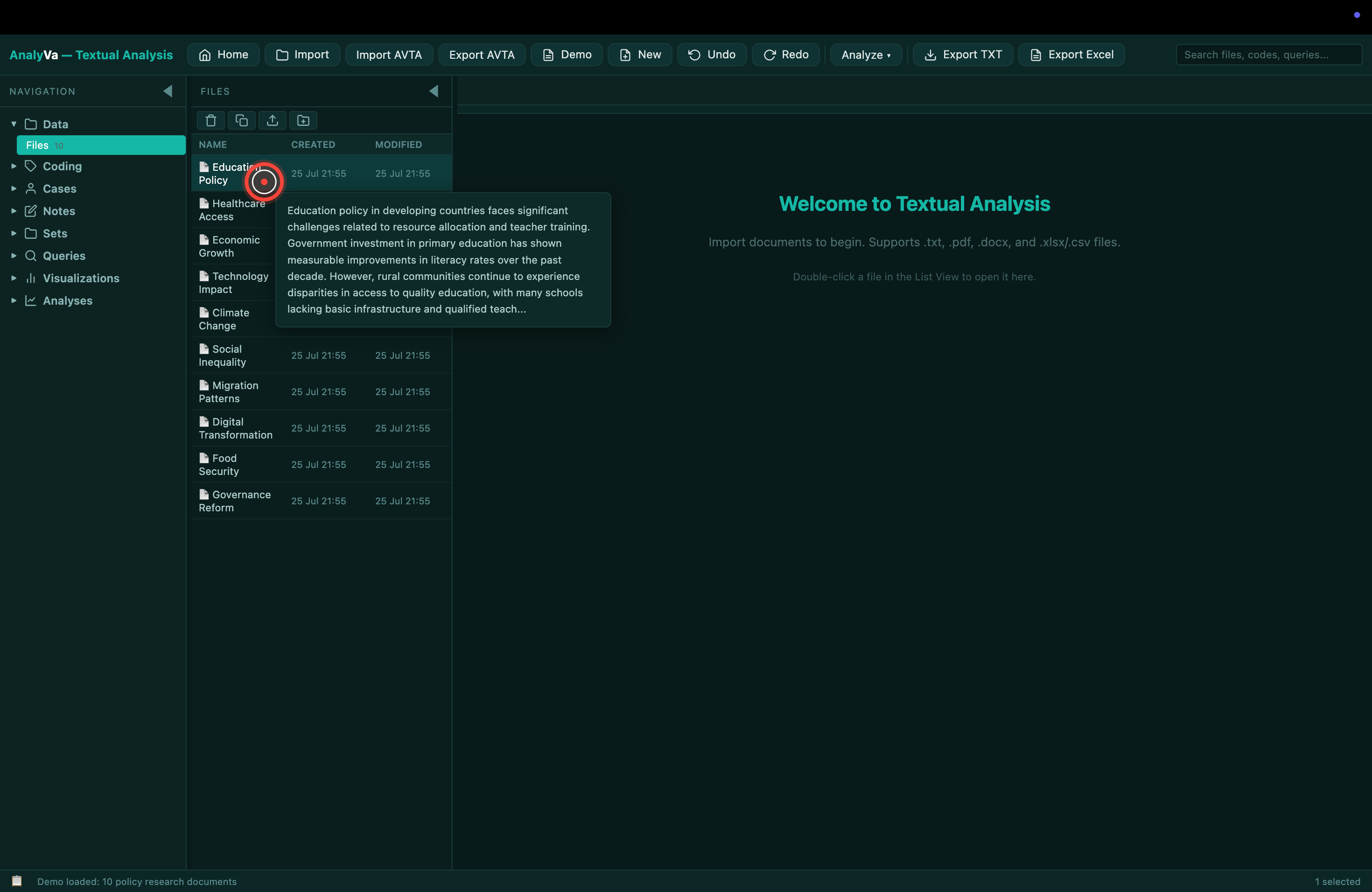
<p><strong>Step 5 — Click a document to open it.</strong>
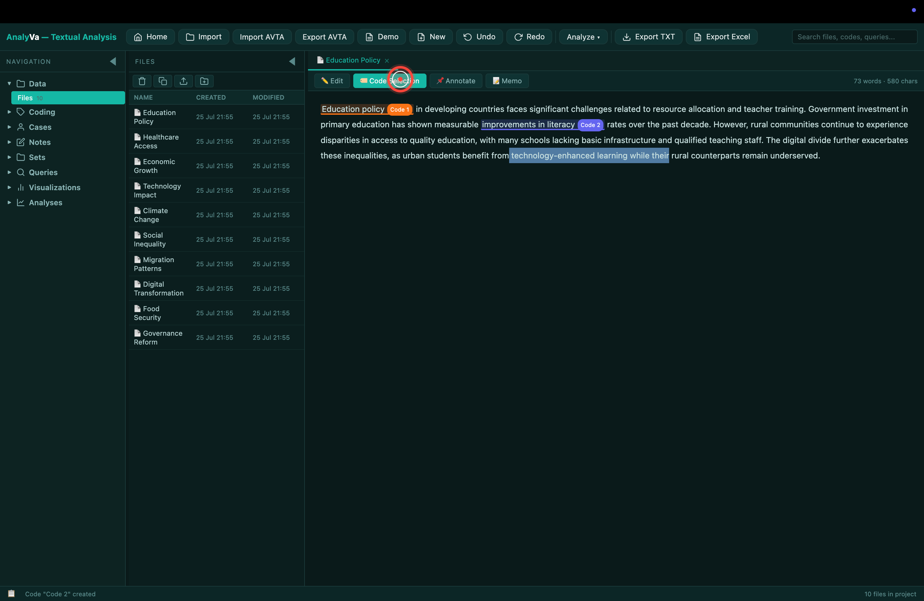
The right pane opens the document with word and character counts in
the top-right, plus four action buttons: <strong>Edit</strong>, <strong>Code Selection</strong>,
<strong>Annotate</strong>, <strong>Memo</strong>.</p>

<p><img src="/blog/images/analyva-coding-05.png" alt="A document open on the right, ready to be coded" /></p>

<p><strong>Step 6 — Skim the text before you start coding.</strong>
Read the document once end-to-end before annotating anything. Codes
built from a first pass through unfamiliar material tend to fragment
the theme; codes built from a second pass tend to organise it.</p>

<p><img src="/blog/images/analyva-coding-06.png" alt="Document text ready for reading" /></p>

<h2 id="coding-text">Coding text</h2>

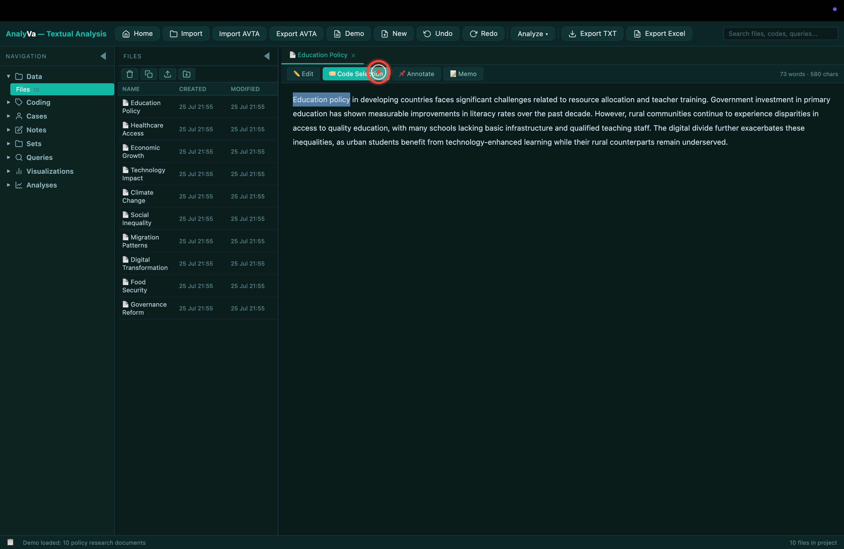
<p><strong>Step 7 — Highlight a passage you want to code.</strong>
Click and drag to select the text — a word, a phrase, a full paragraph.</p>

<p><img src="/blog/images/analyva-coding-07.png" alt="Text highlighted in the document viewer" /></p>

<p><strong>Step 8 — Click <em>Code Selection</em> in the toolbar above the document.</strong>
Or right-click the highlighted text and pick <em>Code Selection</em> from
the context menu.</p>

<p><img src="/blog/images/analyva-coding-08.png" alt="Code Selection button in the toolbar" /></p>

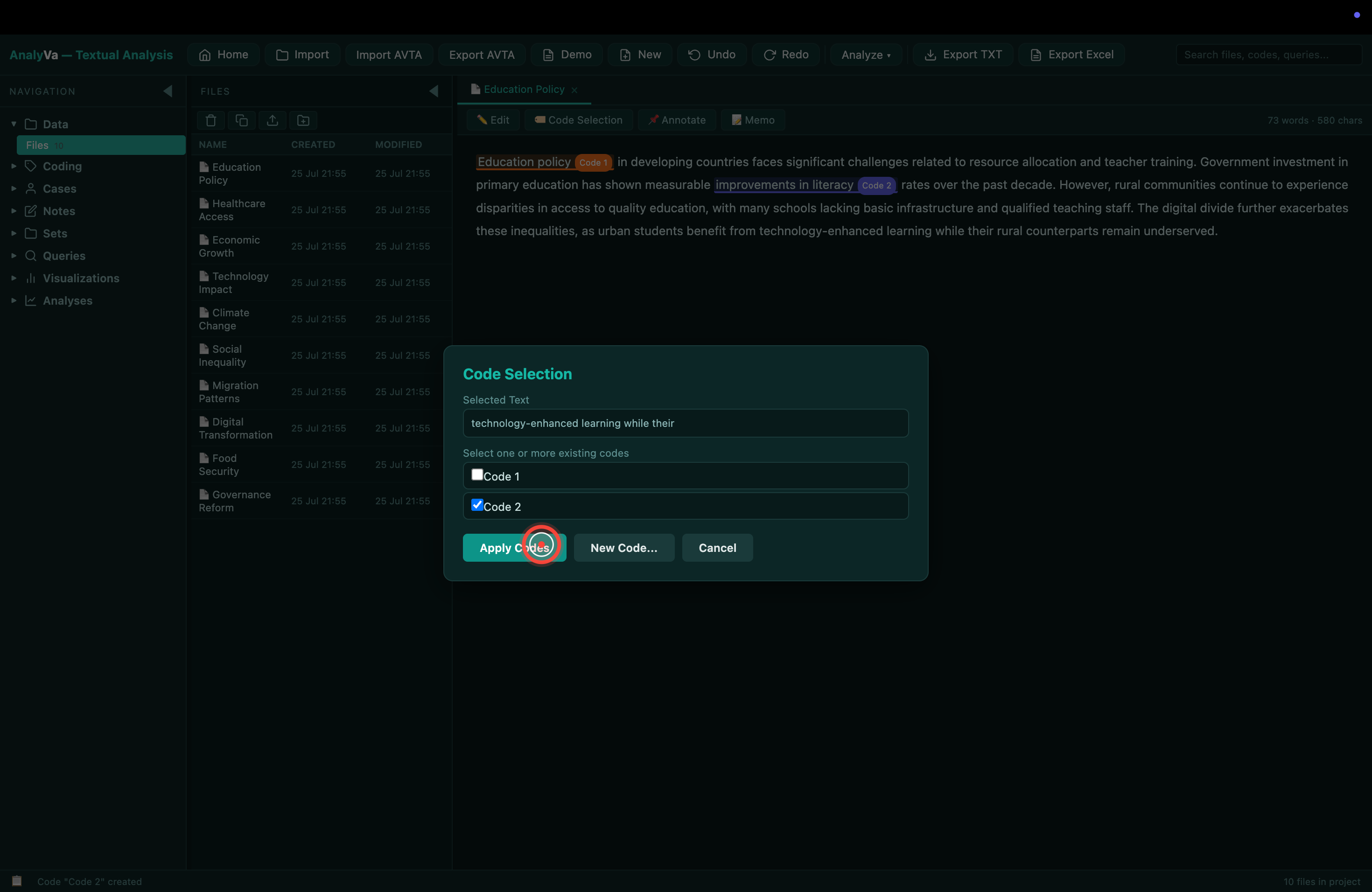
<p><strong>Step 9 — The Code Selection dialog opens.</strong>
It shows the selected text, plus a list of any existing codes you can
apply. On a fresh project this list is empty.</p>

<p><img src="/blog/images/analyva-coding-09.png" alt="Code Selection dialog with the selected text and code list" /></p>

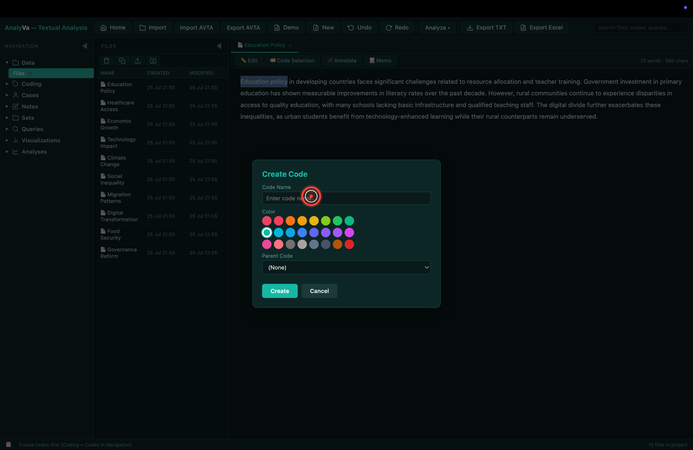
<p><strong>Step 10 — Click <em>New Code</em> to create your first code.</strong>
A prompt asks for the code name — keep it short and descriptive
(<code class="language-plaintext highlighter-rouge">resource_scarcity</code>, <code class="language-plaintext highlighter-rouge">teacher_training</code>, <code class="language-plaintext highlighter-rouge">digital_divide</code>).</p>

<p><img src="/blog/images/analyva-coding-10.png" alt="New Code button ready to create the first code" /></p>

<p><strong>Step 11 — The code is applied.</strong>
The passage is now marked with a colored highlight and a small chip
naming the code. AnalyVa auto-assigns a colour so each code stays
visually distinct.</p>

<p><img src="/blog/images/analyva-coding-11.png" alt="First code applied — highlighted passage with code chip" /></p>

<p><strong>Step 12 — Apply the same code again to a new passage.</strong>
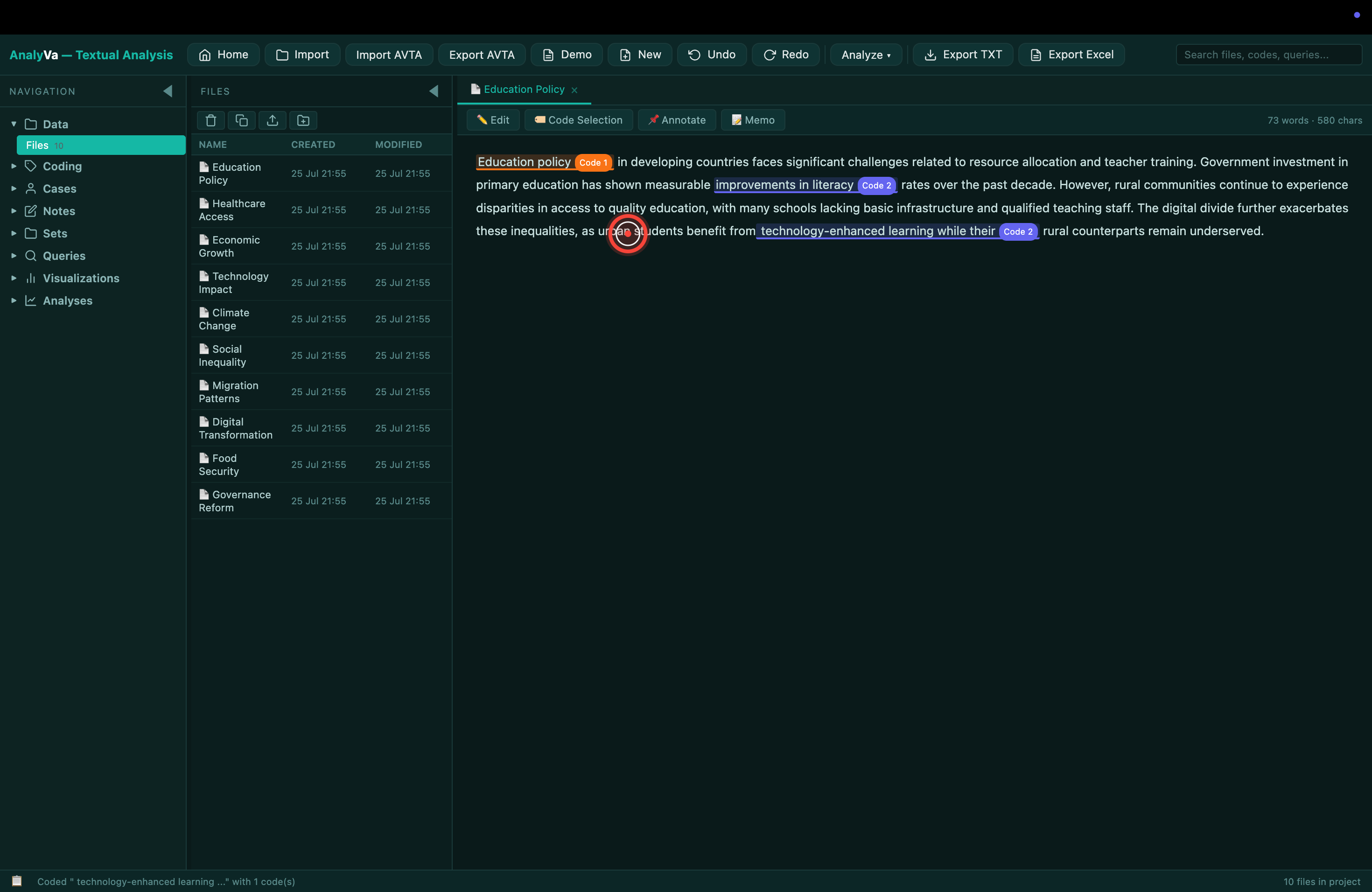
Highlight another chunk of text, open Code Selection, tick the box
next to your existing code, and click <strong>Apply Codes</strong>. The passage
picks up the same colour as before.</p>

<p><img src="/blog/images/analyva-coding-12.png" alt="Second passage tagged with the same code" /></p>

<p><strong>Step 13 — Create additional codes as new themes emerge.</strong>
Grounded-theory-style coding grows the codebook as you read. New
concept? New code. Same concept as before? Reuse the existing code.</p>

<p><img src="/blog/images/analyva-coding-13.png" alt="Multiple codes visible on the same document" /></p>

<p><strong>Step 14 — Work across multiple documents.</strong>
Codes are project-wide — a code you created on the Education Policy
document is available on every other document in the corpus. This is
where the value of a systematic codebook pays off: consistent codes
across documents let you query them together later.</p>

<p><img src="/blog/images/analyva-coding-14.png" alt="Coding continues on a second document, reusing existing codes" /></p>

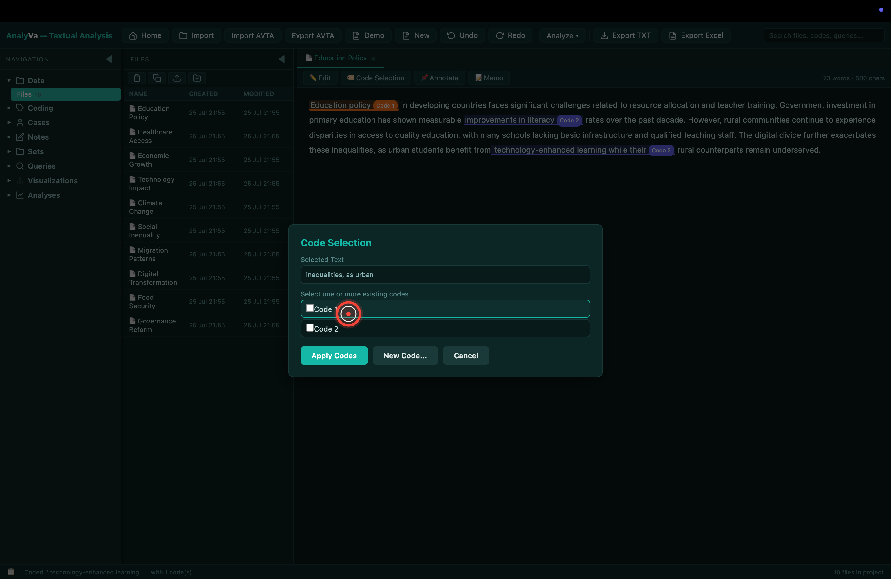
<p><strong>Step 15 — Overlap and nesting are allowed.</strong>
A single passage can carry multiple codes. This is often the point of
qualitative coding — a paragraph about “<em>teachers in rural schools</em>”
might be tagged both <code class="language-plaintext highlighter-rouge">teacher_training</code> and <code class="language-plaintext highlighter-rouge">rural_inequality</code>.</p>

<p><img src="/blog/images/analyva-coding-15.png" alt="A passage with two overlapping codes" /></p>

<h2 id="reviewing-what-you-have-coded">Reviewing what you have coded</h2>

<p><strong>Step 16 — Open <em>Coding</em> in the left Navigation sidebar.</strong>
The Coding section lists every code in the project, how many segments
it appears in, and across how many documents.</p>

<p><img src="/blog/images/analyva-coding-16.png" alt="Coding view in the sidebar with the code list" /></p>

<p><strong>Step 17 — Click a code to see every segment tagged with it.</strong>
The right pane switches to a <strong>Coded Segments</strong> view — one row per
segment, showing the document, the surrounding context, and links
back to the original position. This is the review step where you
notice inconsistencies (segments that were mis-coded, codes that
should be merged, etc.).</p>

<p><img src="/blog/images/analyva-coding-17.png" alt="Coded Segments view for a single code" /></p>

<p><strong>Step 18 — Rename, merge, or delete codes.</strong>
Right-click a code in the Coding sidebar to rename it (updates every
segment automatically), merge two codes into one, or delete a code
(with a warning about the segments it will affect).</p>

<p><img src="/blog/images/analyva-coding-18.png" alt="Code management right-click menu" /></p>

<p><strong>Step 19 — Add memos to codes and to segments.</strong>
Codes and individual segments both accept <strong>memos</strong> — free-text
reflection about what you were thinking when you tagged something.
Reviewers love these; future-you loves them even more.</p>

<p><img src="/blog/images/analyva-coding-19.png" alt="Memo attached to a code" /></p>

<p><strong>Step 20 — Add cases if your corpus has speakers or interviewees.</strong>
The <strong>Cases</strong> section links documents to sources (interview
respondents, workshop groups, focus groups). This is what lets you
later ask “did female respondents talk about X more than male
respondents?” — a demographic query on the qualitative data.</p>

<p><img src="/blog/images/analyva-coding-20.png" alt="Cases view for linking documents to respondents" /></p>

<h2 id="running-analyses-on-the-coded-corpus">Running analyses on the coded corpus</h2>

<p><strong>Step 21 — Open <em>Analyses</em> in the sidebar.</strong>
This is where AnalyVa’s quantitative-qualitative bridge shows up.
Every code-count, code-cooccurrence, and code-by-case matrix is one
click away.</p>

<p><img src="/blog/images/analyva-coding-21.png" alt="Analyses menu options for the coded corpus" /></p>

<p><strong>Step 22 — Run a <em>Codes-by-cases</em> matrix.</strong>
For every code and every case, the matrix shows how many segments
that case contributed to that code. Instantly reveals which codes are
concentrated in which respondents, and which are broadly distributed.</p>

<p><img src="/blog/images/analyva-coding-22.png" alt="Codes-by-cases matrix output" /></p>

<p><strong>Step 23 — Run a <em>Code co-occurrence</em> analysis.</strong>
For every pair of codes, this counts how often they appear in the
same segment — the qualitative analogue of correlation. High
co-occurrence between two codes often points to a merger or a
higher-order theme.</p>

<p><img src="/blog/images/analyva-coding-23.png" alt="Code co-occurrence table" /></p>

<p><strong>Step 24 — Open <em>Visualizations</em> for the graphical view.</strong>
Word clouds, code frequency charts, code hierarchies. Useful in
manuscript figures and as a first-look sanity check on the code
distribution.</p>

<p><img src="/blog/images/analyva-coding-24.png" alt="Visualizations menu for the coded corpus" /></p>

<p><strong>Step 25 — Export.</strong>
The top toolbar has <strong>Export TXT</strong>, <strong>Export Excel</strong>, and
<strong>Export AVTA</strong> (AnalyVa’s own portable format for a full project
including codes, memos, and cases). Export AVTA when handing the
project to a collaborator; export Excel when moving a code frequency
table into a paper.</p>

<p><img src="/blog/images/analyva-coding-25.png" alt="Export options in the top toolbar" /></p>

<h2 id="what-to-remember">What to remember</h2>

<p>Qualitative coding in AnalyVa follows the same four-stage rhythm as
in NVivo, MAXQDA, or Atlas.ti:</p>

<ol>
  <li><strong>Import</strong> your documents (or use the demo corpus first).</li>
  <li><strong>Code</strong> passages — one at a time, growing your codebook as new
themes emerge, applying existing codes to reuse them.</li>
  <li><strong>Review</strong> every code’s segments in the Coding sidebar. Rename,
merge, delete as needed.</li>
  <li><strong>Analyse</strong> via Codes-by-cases, Co-occurrence, or Visualizations.</li>
</ol>

<p>The two things AnalyVa gives you that stand-alone qualitative tools
do not: your quantitative variables are still available in the other
workspace (switch anytime via <strong>Home</strong>), and you get an integrated
Export AVTA format that packages everything for peer review or
collaborator handoff.</p>]]></content><author><name>Abdelouahd Bouzar</name><email>support@analyva.com</email></author><category term="Qualitative Analysis" /><category term="analyva" /><category term="qualitative" /><category term="coding" /><category term="textual analysis" /><summary type="html"><![CDATA[A full walkthrough of qualitative text analysis in AnalyVa — loading documents, highlighting passages, creating codes, applying them, and reviewing coded segments across the corpus.]]></summary><media:thumbnail xmlns:media="http://search.yahoo.com/mrss/" url="https://analyva.com/blog/images/cover-coding.svg" /><media:content medium="image" url="https://analyva.com/blog/images/cover-coding.svg" xmlns:media="http://search.yahoo.com/mrss/" /></entry><entry><title type="html">Reverse Coding, Recoding &amp;amp; Changing Variable Types in AnalyVa</title><link href="https://analyva.com/blog/recoding-and-variable-types-in-analyva/" rel="alternate" type="text/html" title="Reverse Coding, Recoding &amp;amp; Changing Variable Types in AnalyVa" /><published>2026-07-29T00:00:00+00:00</published><updated>2026-07-29T00:00:00+00:00</updated><id>https://analyva.com/blog/recoding-and-variable-types-in-analyva</id><content type="html" xml:base="https://analyva.com/blog/recoding-and-variable-types-in-analyva/"><![CDATA[<p>Between importing a dataset and running an analysis sits a step almost
every applied paper glosses over: <strong>data preparation.</strong> Are your Likert
items typed as ordinal or scale? Did you remember to reverse-code the
three negatively-worded items in the rumination scale? Did you
collapse the age variable into meaningful bands?</p>

<p>AnalyVa handles all of these inside a single <strong>Data → Variable View</strong>
panel — one that will feel familiar if you have ever used SPSS.</p>

<h2 id="getting-to-the-data-view">Getting to the Data view</h2>

<p><strong>Step 1 — Click <em>Data</em> in the top toolbar.</strong>
Once your dataset is imported, the <strong>Data</strong> button (rightmost cluster,
next to Export) opens a full-screen data browser.</p>

<p><img src="/blog/images/analyva-recoding-01.png" alt="The Data button highlighted in the top toolbar" /></p>

<p><strong>Step 2 — Switch to <em>Variable View</em>.</strong>
The Data browser has two tabs: <strong>Data View</strong> (rows and cells, like a
spreadsheet) and <strong>Variable View</strong> (one row per variable, listing
type, label, values, missing-value codes).</p>

<p><img src="/blog/images/analyva-recoding-02.png" alt="The Variable View tab in the Data browser" /></p>

<p>Every subsequent operation in this post happens in Variable View.</p>

<h2 id="task-1--change-the-type-of-a-single-variable">Task 1 — Change the type of a single variable</h2>

<p>By default, AnalyVa infers types from the imported data (numeric →
Scale, text → Nominal, etc.). To change a variable’s type:</p>

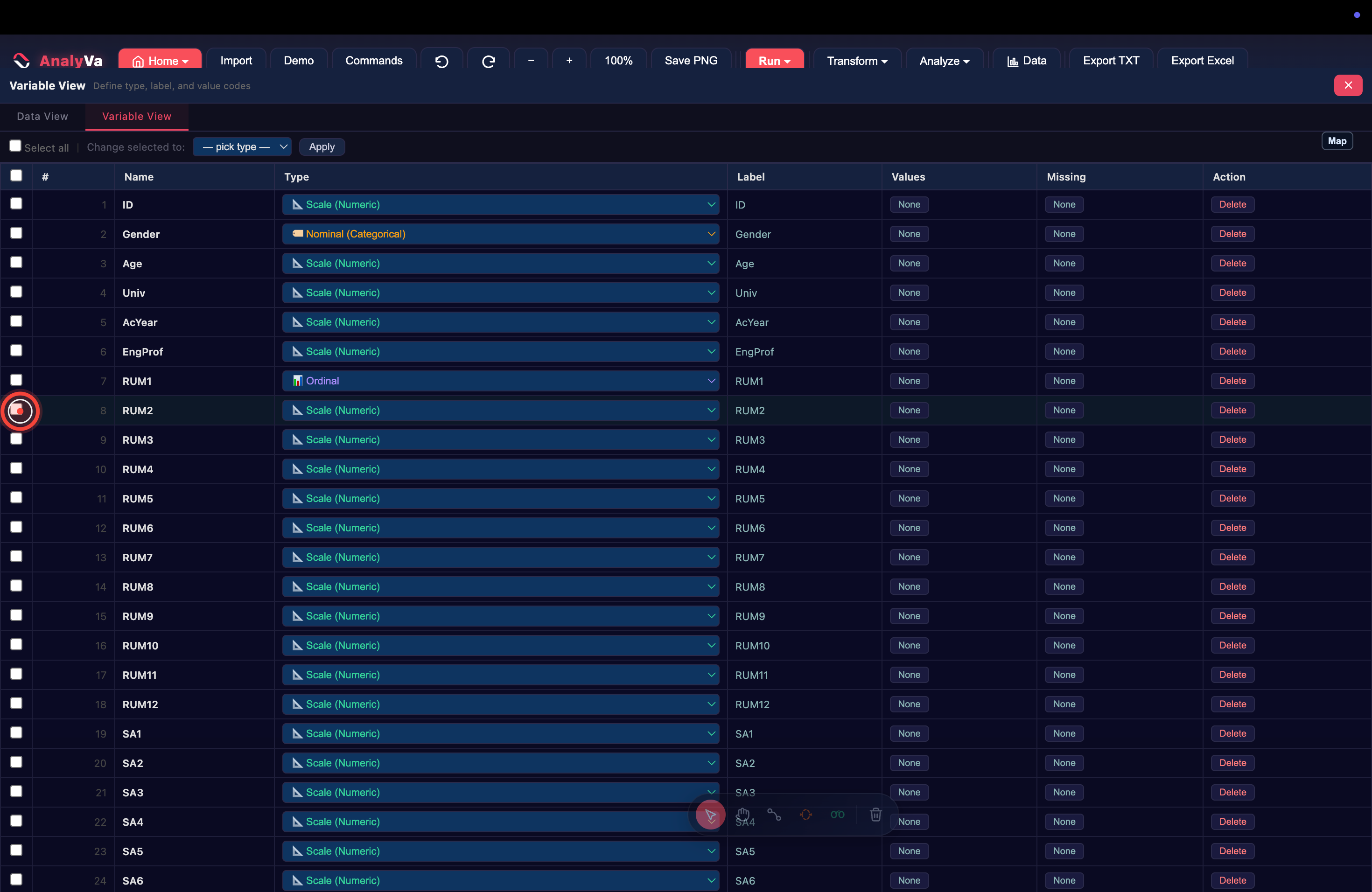
<p><strong>Step 3 — Click the Type dropdown for the row you want to change.</strong>
You will see three options: <strong>Scale (Numeric)</strong>, <strong>Nominal
(Categorical)</strong>, and <strong>Ordinal</strong>.</p>

<p><img src="/blog/images/analyva-recoding-03.png" alt="The Type dropdown open on a single row" /></p>

<p><strong>Step 4 — Pick the appropriate type.</strong>
As a quick reminder:</p>

<ul>
  <li><strong>Scale</strong> — interval or ratio (age in years, income, exam score).</li>
  <li><strong>Nominal</strong> — unordered categories (gender, country, brand).</li>
  <li><strong>Ordinal</strong> — ordered categories with unequal spacing (Likert
responses 1–5, education level).</li>
</ul>

<p>Most survey scale items are technically ordinal, but many analyses
treat them as scale in practice. Pick the type that matches the
analysis you plan to run.</p>

<p><img src="/blog/images/analyva-recoding-04.png" alt="The variable's new type applied" /></p>

<p><strong>Step 5 — The change is instant.</strong>
No Save button, no confirmation dialog. AnalyVa applies the type
change immediately.</p>

<p><img src="/blog/images/analyva-recoding-05.png" alt="The updated Variable View" /></p>

<p><strong>Step 6 — Sanity-check downstream.</strong>
Every row shows a small type-icon on the left of the Type dropdown —
scale, nominal, or ordinal. Scan the column to catch any variables
still typed wrong.</p>

<p><img src="/blog/images/analyva-recoding-06.png" alt="The Variable View listing all typed variables" /></p>

<h2 id="task-2--change-the-type-of-many-variables-at-once">Task 2 — Change the type of many variables at once</h2>

<p>If you just imported a 60-item questionnaire, changing types one row
at a time is tedious. AnalyVa has a bulk-change mode.</p>

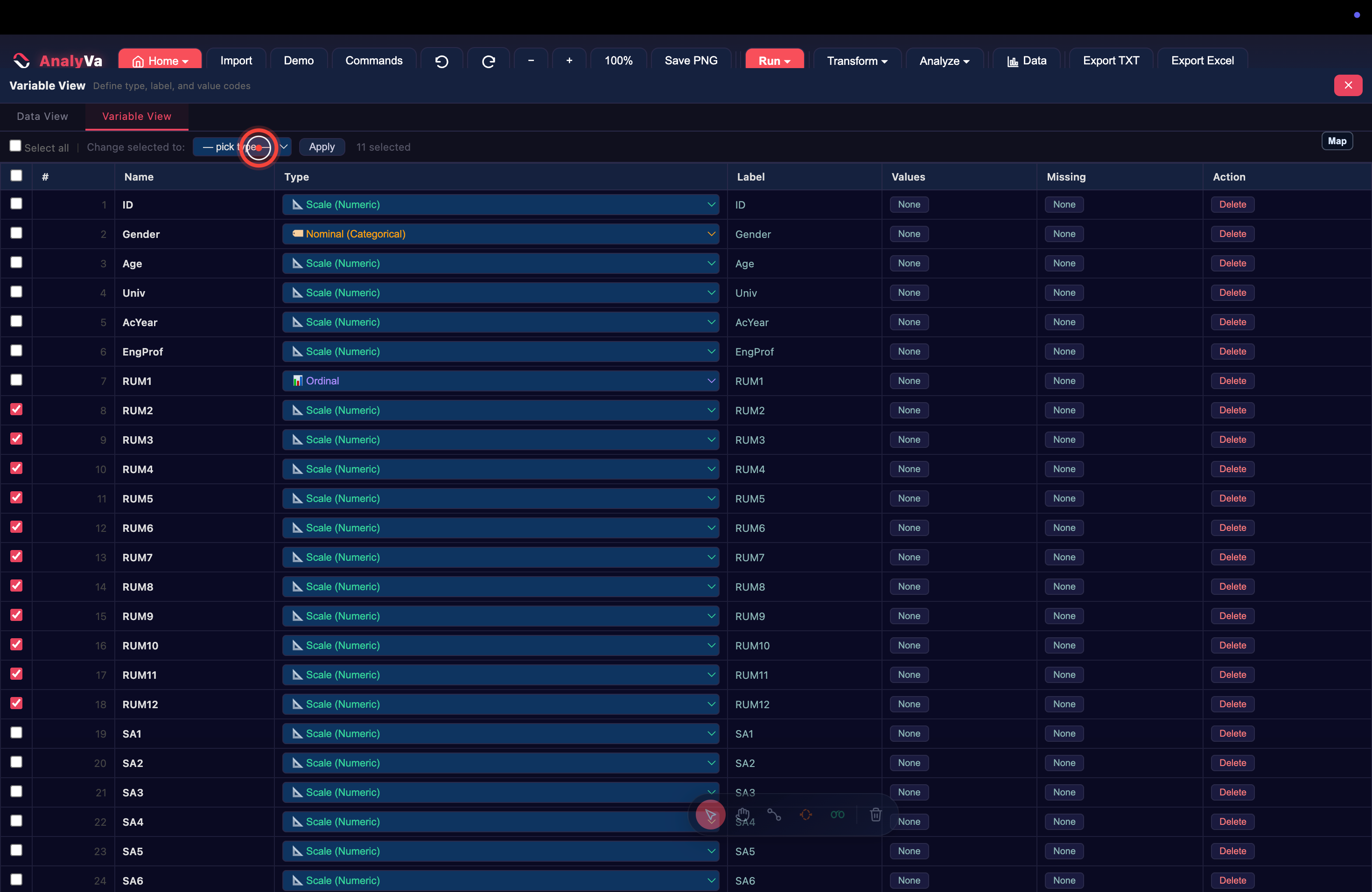
<p><strong>Step 7 — Tick the checkbox on each row you want to change.</strong>
The leftmost column is a selection checkbox. Ticked rows highlight
red.</p>

<p><img src="/blog/images/analyva-recoding-07.png" alt="Multiple rows selected for bulk change" /></p>

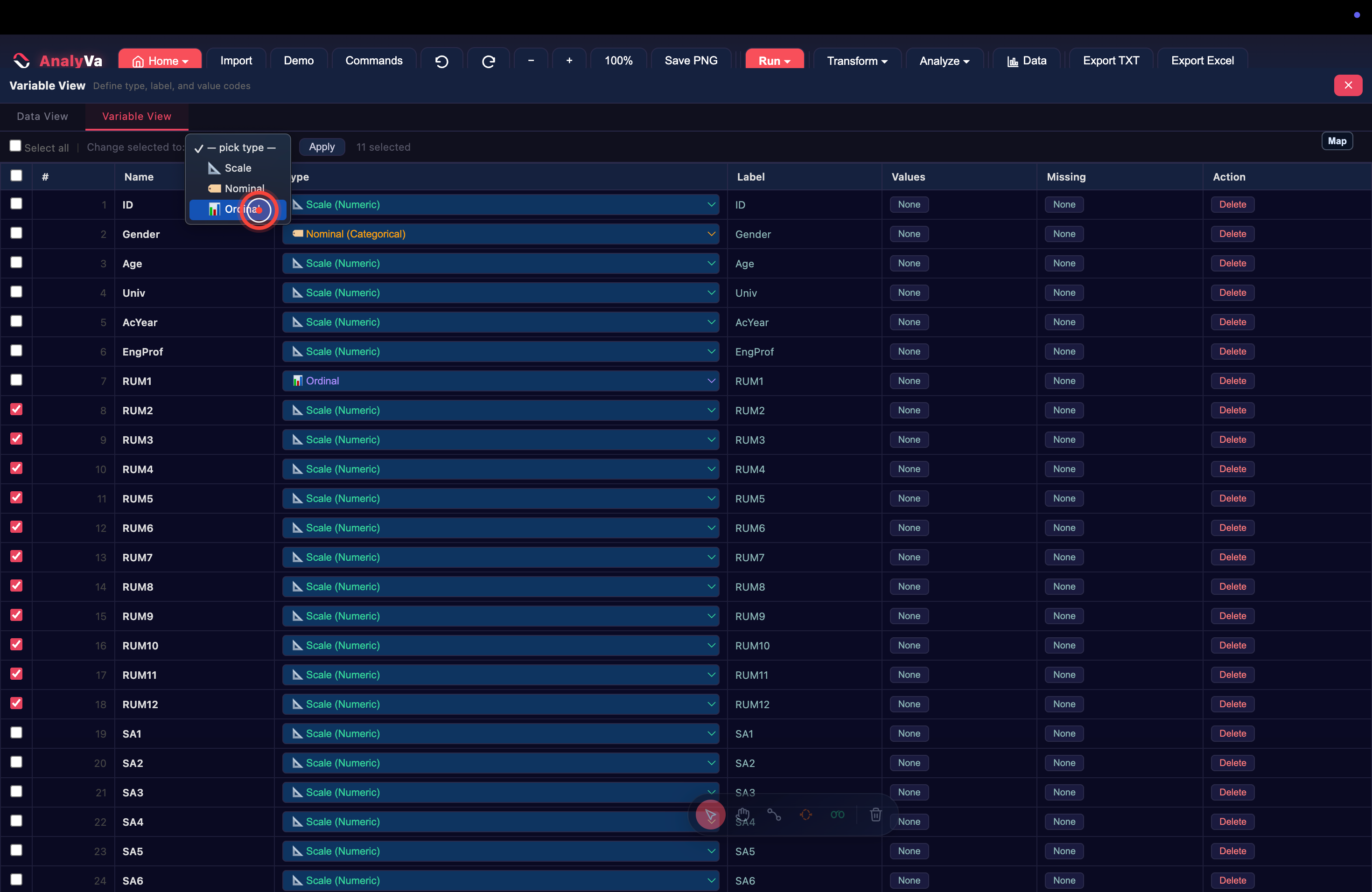
<p><strong>Step 8 — Pick the new type from <em>Change selected to</em> and click
<em>Apply</em>.</strong>
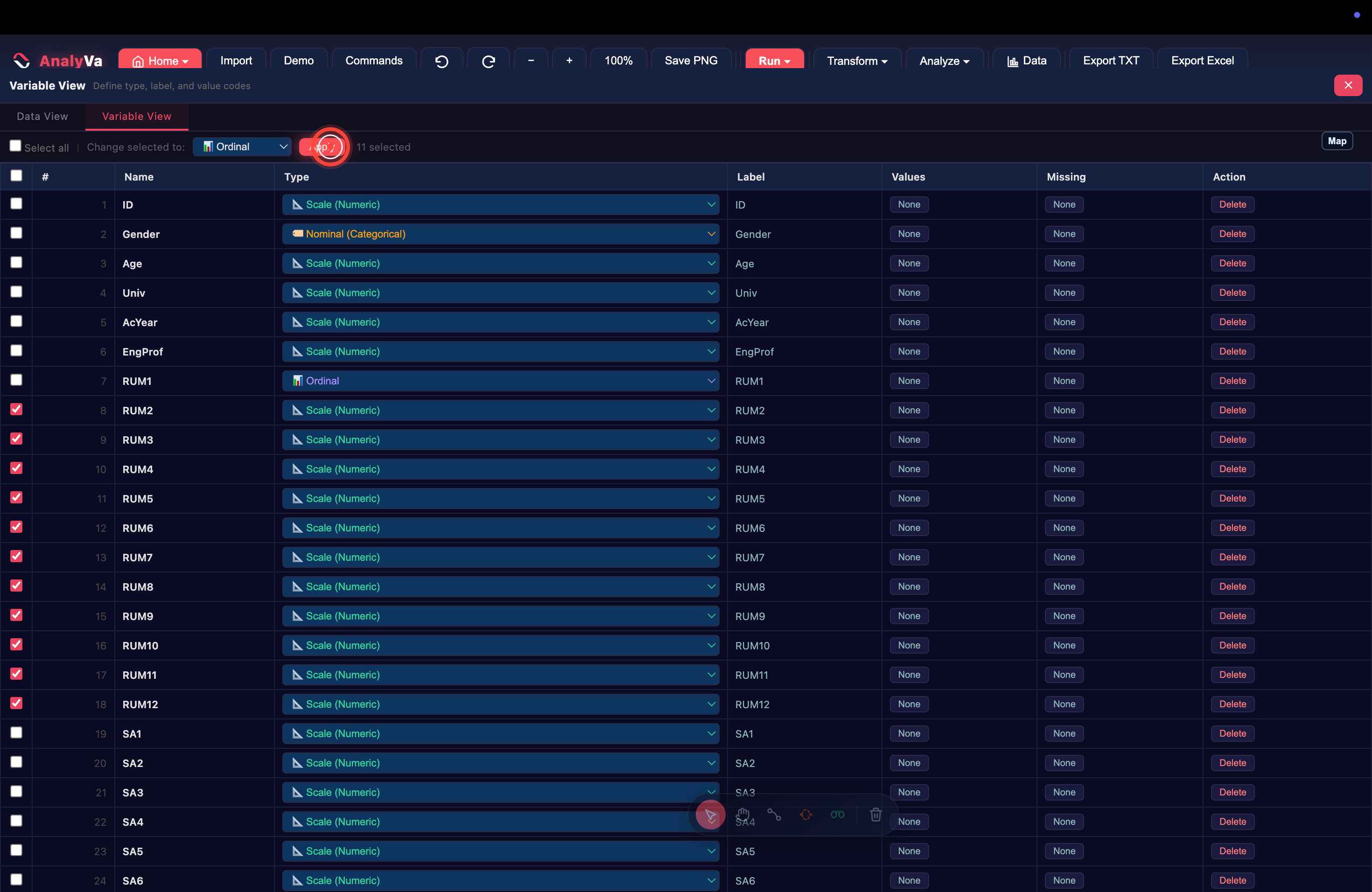
At the top of the Variable View, next to the <em>Select all</em> checkbox, a
dropdown appears with <code class="language-plaintext highlighter-rouge">— pick type —</code>. Choose Scale, Nominal, or
Ordinal. A counter tells you how many rows the change will affect
(here: <code class="language-plaintext highlighter-rouge">11 selected</code>). Click <strong>Apply</strong> and every selected row updates
at once.</p>

<p><img src="/blog/images/analyva-recoding-08.png" alt="Bulk type-change to Ordinal with 11 variables selected" /></p>

<h2 id="task-3--reverse-code-a-scale">Task 3 — Reverse-code a scale</h2>

<p>Well-designed questionnaires often include <strong>negatively-worded items</strong>
to catch inattentive respondents. Before analysing the scale, those
items must be reverse-coded — a <code class="language-plaintext highlighter-rouge">5</code> on a 5-point Likert flips to <code class="language-plaintext highlighter-rouge">1</code>,
a <code class="language-plaintext highlighter-rouge">4</code> flips to <code class="language-plaintext highlighter-rouge">2</code>, and so on.</p>

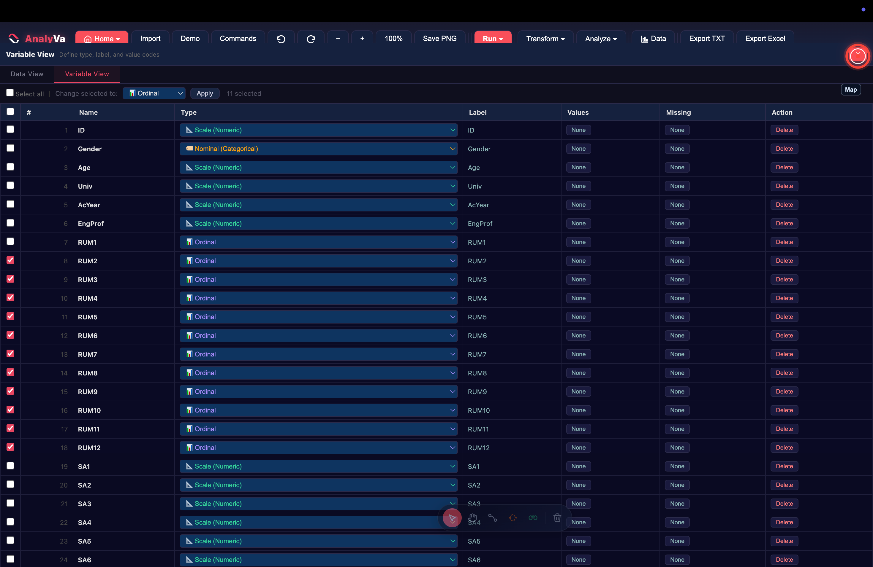
<p><strong>Step 9 — Confirm the recoding applied.</strong>
The header shows a confirmation like <em>“11 variables set to ordinal”</em>
so you know the previous step succeeded.</p>

<p><img src="/blog/images/analyva-recoding-09.png" alt="Confirmation that the bulk change was applied" /></p>

<p><strong>Step 10 — Return to the main workspace.</strong>
Close the Data view or press <strong>Esc</strong>. The sidebar now shows every
variable in the dataset.</p>

<p><img src="/blog/images/analyva-recoding-10.png" alt="Back on the main workspace with the variables listed" /></p>

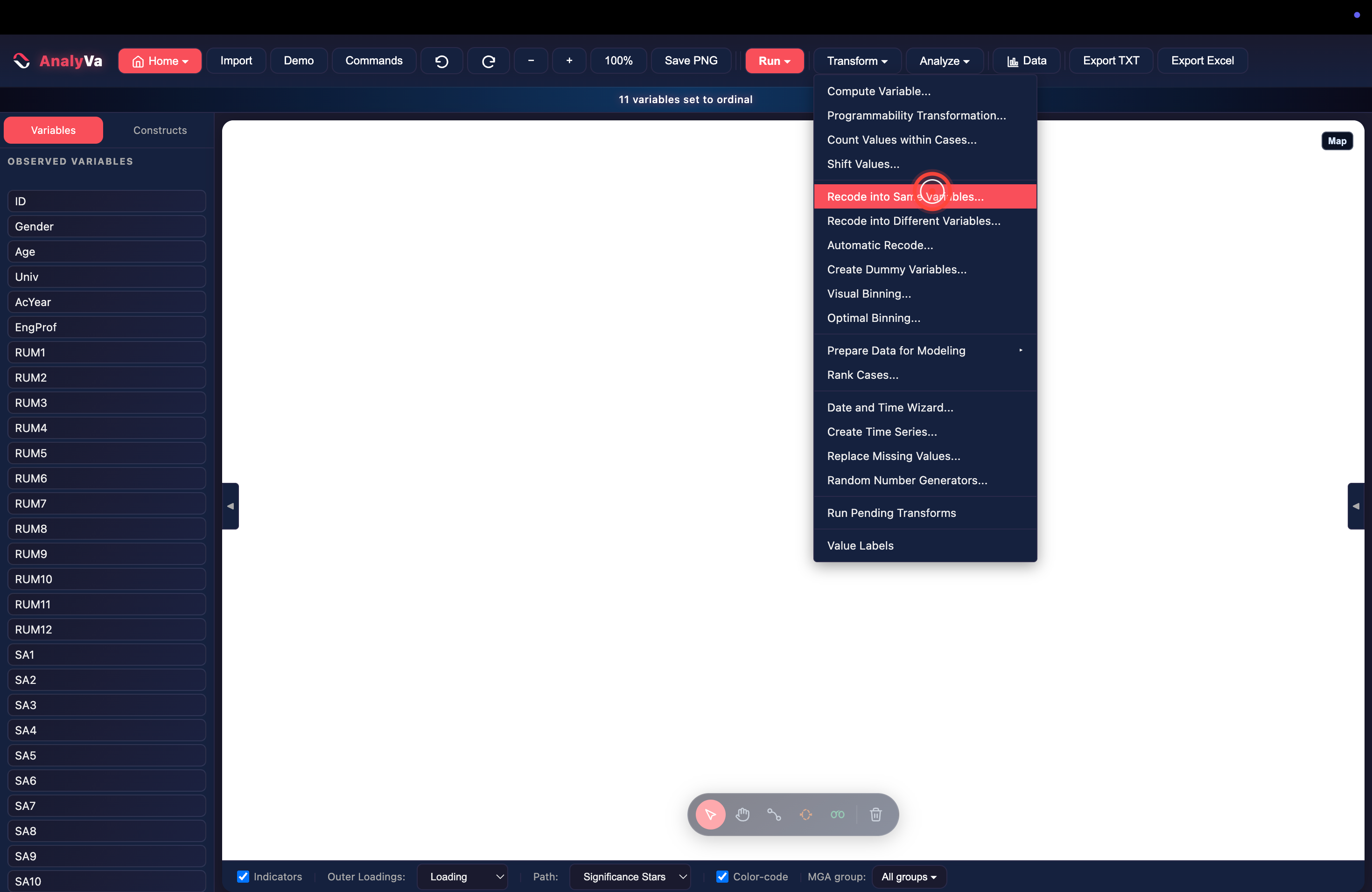
<p><strong>Step 11 — Open <em>Transform → Recode into Same Variables</em>.</strong>
The Transform menu at the top of the app holds every data-manipulation
command. <strong>Recode into Same Variables</strong> rewrites values in place —
useful for reverse-coding. <strong>Recode into Different Variables</strong> creates
a new column with the recoded values — safer when you want to keep
the original.</p>

<p><img src="/blog/images/analyva-recoding-11.png" alt="Transform menu with Recode into Same Variables highlighted" /></p>

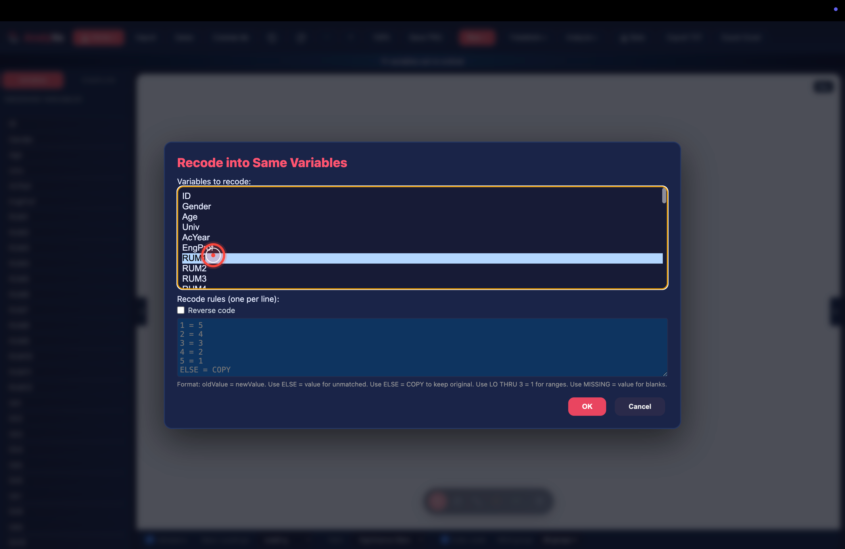
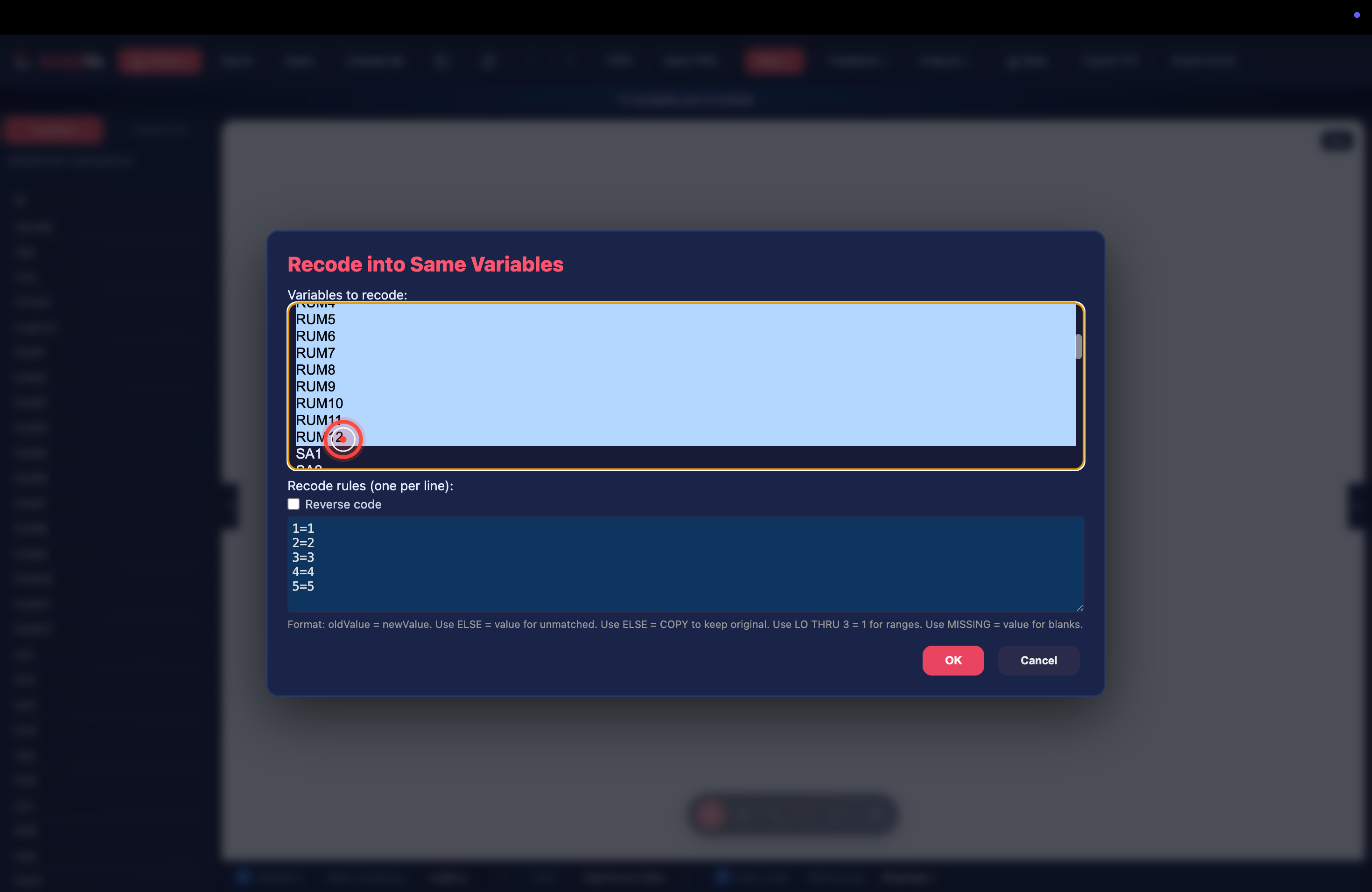
<p><strong>Step 12 — The Recode dialog opens.</strong>
Select the variables you want to reverse-code (Cmd/Ctrl-click for
multiple, or Shift-click for a range).</p>

<p><img src="/blog/images/analyva-recoding-12.png" alt="The Recode dialog with variables to recode listed" /></p>

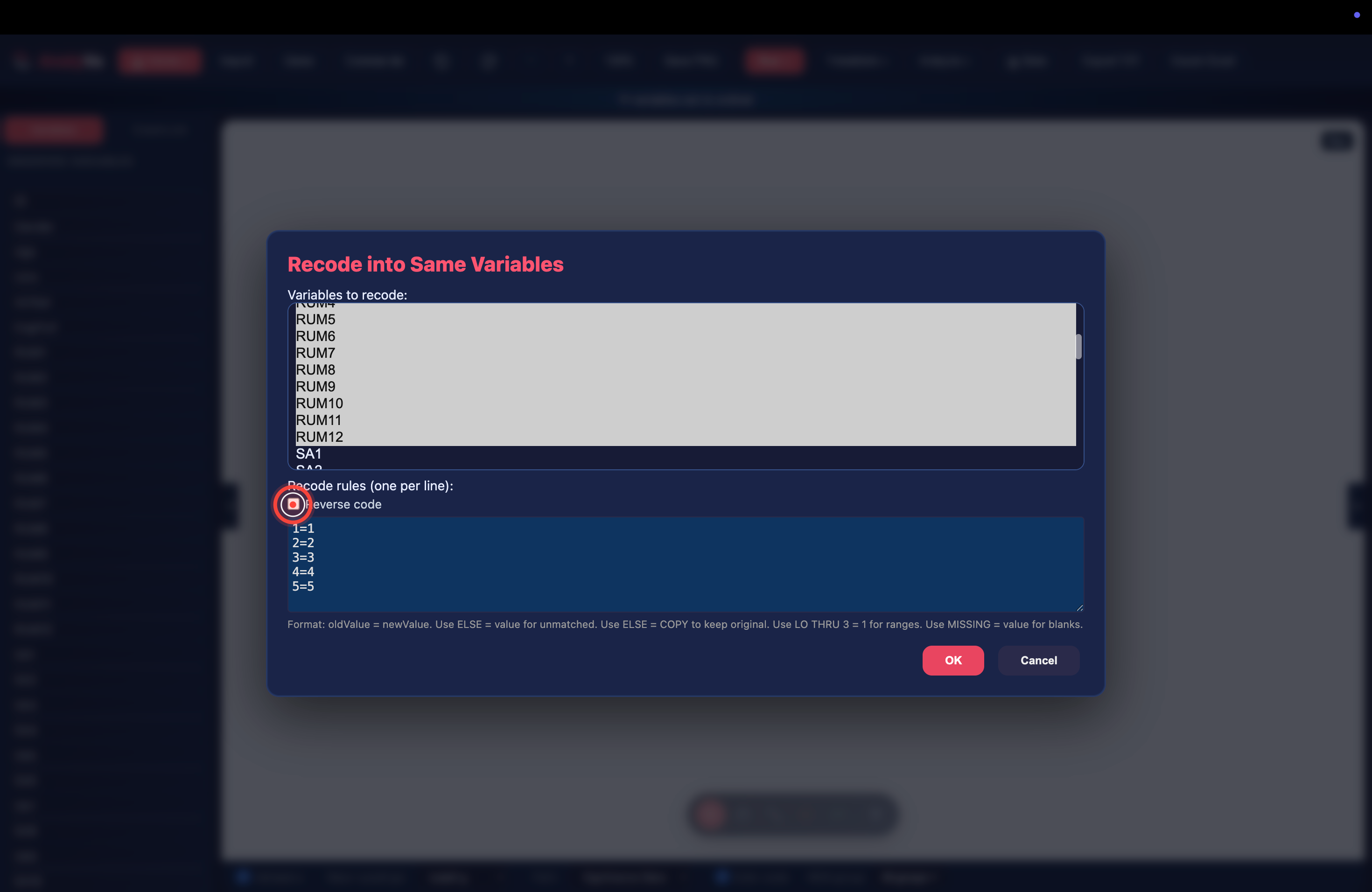
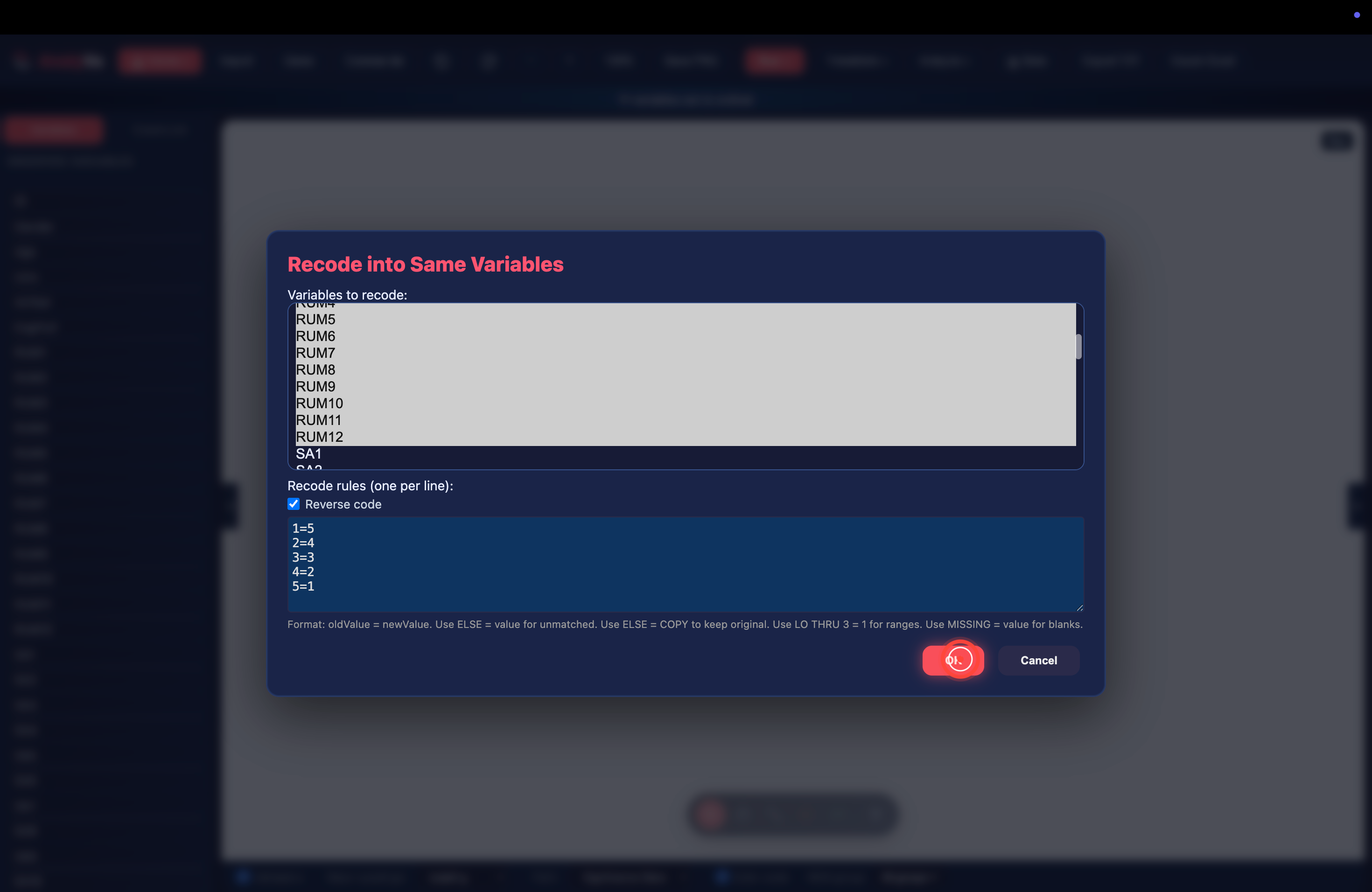
<p><strong>Step 13 — Tick <em>Reverse code</em> — or write the rules manually.</strong>
Two ways to reverse-code:</p>

<ul>
  <li><strong>Fastest</strong> — tick the <strong>Reverse code</strong> checkbox. AnalyVa infers
the scale from the selected variables and generates the rules
automatically (e.g. <code class="language-plaintext highlighter-rouge">1=5</code>, <code class="language-plaintext highlighter-rouge">2=4</code>, <code class="language-plaintext highlighter-rouge">3=3</code>, <code class="language-plaintext highlighter-rouge">4=2</code>, <code class="language-plaintext highlighter-rouge">5=1</code>).</li>
  <li><strong>Manual</strong> — write the rules directly in the Recode rules box, one
per line, using the format <code class="language-plaintext highlighter-rouge">oldValue = newValue</code>. Special tokens:
    <ul>
      <li><code class="language-plaintext highlighter-rouge">LO THRU 3 = 1</code> — recode “lowest through 3” as 1 (range).</li>
      <li><code class="language-plaintext highlighter-rouge">ELSE = COPY</code> — keep original for anything not matched.</li>
      <li><code class="language-plaintext highlighter-rouge">MISSING = 99</code> — assign a code to blank cells.</li>
    </ul>
  </li>
</ul>

<p><img src="/blog/images/analyva-recoding-13.png" alt="The Recode rules box with the Reverse code checkbox" /></p>

<p><strong>Step 14 — Click <em>OK</em>.</strong>
The recode is applied in place. Back in Data View you can spot-check
that the values flipped correctly.</p>

<p><img src="/blog/images/analyva-recoding-14.png" alt="Recode applied — values flipped in place" /></p>

<p><strong>Step 15 — Recompute any composite scores.</strong>
If you already built mean/sum composites from the raw items via
<em>Transform → Compute Variable</em>, they are now stale. Delete the old
composites and recompute them so the reverse-coded values propagate.
This is the single most common data-prep bug — the reverse-code runs
but downstream composites still reflect the un-reversed values.</p>

<p><img src="/blog/images/analyva-recoding-15.png" alt="Data view after the recode" /></p>

<h2 id="the-order-that-matters">The order that matters</h2>

<p>For any dataset arriving fresh from a survey platform, the safest
sequence is:</p>

<ol>
  <li><strong>Import</strong> the data.</li>
  <li><strong>Fix variable types</strong> in Variable View (bulk-change if possible).</li>
  <li><strong>Reverse-code</strong> any negatively-worded items via Recode into Same
Variables + the Reverse code checkbox.</li>
  <li><strong>Compute composite scores</strong> with Transform → Compute Variable.</li>
  <li><strong>Only then run analyses</strong> on the composites.</li>
</ol>

<p>Skip a step and every downstream result inherits the mistake.</p>]]></content><author><name>Abdelouahd Bouzar</name><email>support@analyva.com</email></author><category term="Data Preparation" /><category term="analyva" /><category term="data preparation" /><category term="recoding" /><summary type="html"><![CDATA[Before you run a single analysis, your data needs to be prepared. Change variable types in bulk, recode responses, and reverse-code negatively worded items — all inside AnalyVa's Data view.]]></summary><media:thumbnail xmlns:media="http://search.yahoo.com/mrss/" url="https://analyva.com/blog/images/cover-recoding.svg" /><media:content medium="image" url="https://analyva.com/blog/images/cover-recoding.svg" xmlns:media="http://search.yahoo.com/mrss/" /></entry><entry><title type="html">AnalyVa’s Command Palette: Every Shortcut You’ll Actually Use</title><link href="https://analyva.com/blog/analyva-command-palette-keyboard-shortcuts/" rel="alternate" type="text/html" title="AnalyVa’s Command Palette: Every Shortcut You’ll Actually Use" /><published>2026-07-27T00:00:00+00:00</published><updated>2026-07-27T00:00:00+00:00</updated><id>https://analyva.com/blog/analyva-command-palette-keyboard-shortcuts</id><content type="html" xml:base="https://analyva.com/blog/analyva-command-palette-keyboard-shortcuts/"><![CDATA[<p>Most people never open the command palette. That is a mistake — it is
the single fastest way to work in AnalyVa. Every command in the app —
including the ones buried three menus deep — is one keystroke away
inside it.</p>

<h2 id="opening-the-palette">Opening the palette</h2>

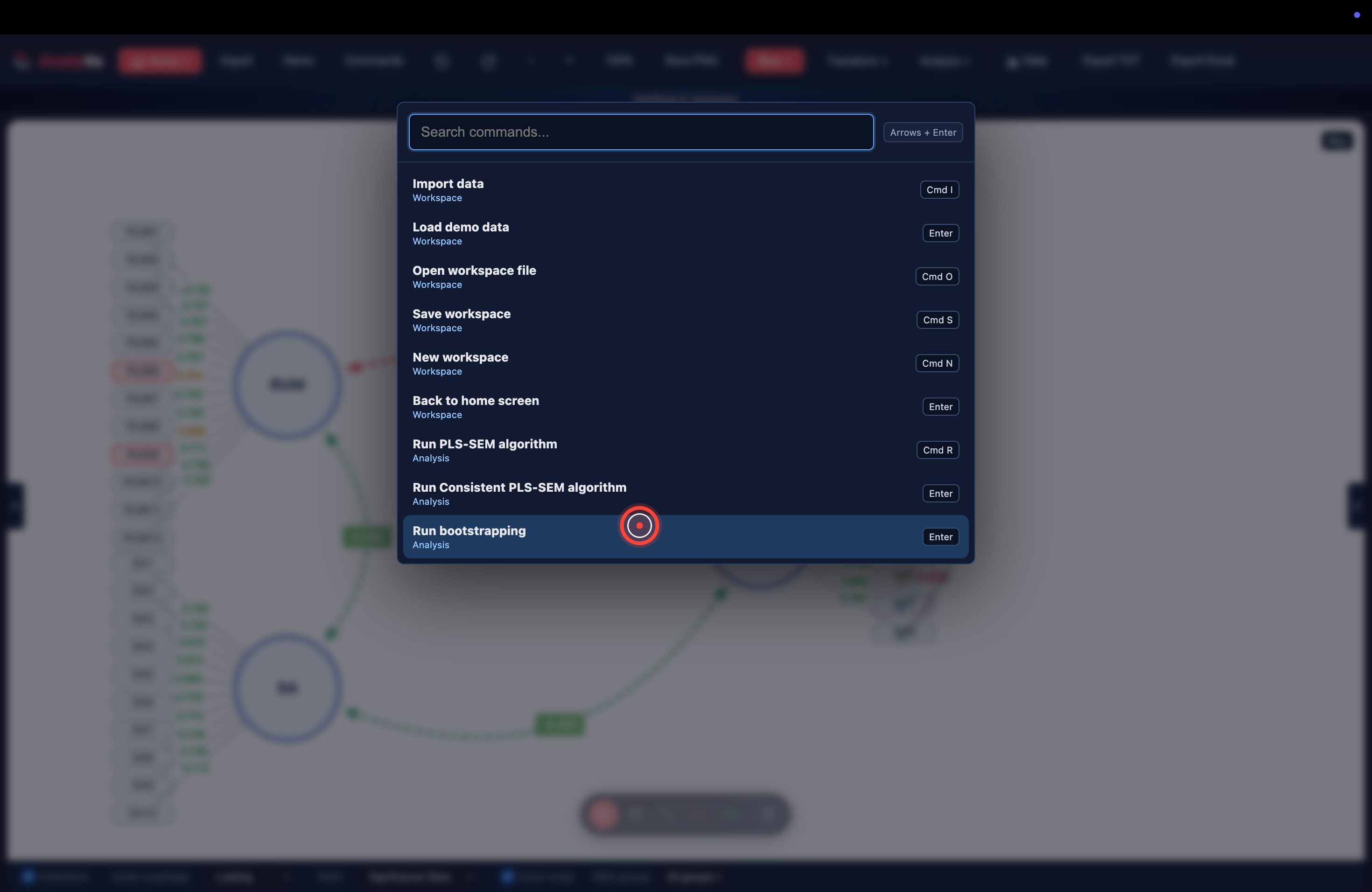
<p>Press <strong>⌘ + K</strong> (macOS) or <strong>Ctrl + K</strong> (Windows/Linux) from anywhere
in the app. A search bar drops from the top. Type the first few
letters of what you want to do — <code class="language-plaintext highlighter-rouge">bootstr</code>, <code class="language-plaintext highlighter-rouge">htmt</code>, <code class="language-plaintext highlighter-rouge">fit</code>, <code class="language-plaintext highlighter-rouge">pca</code> — and
the matching commands filter live. Hit <strong>Enter</strong> to run the top hit,
or use the arrow keys and then Enter.</p>

<p>Close the palette by pressing <strong>Esc</strong> or clicking anywhere outside it.</p>

<h2 id="three-families-of-commands">Three families of commands</h2>

<p>Every command in the palette shows its <strong>category</strong> underneath the
name (Workspace, Analysis, Panels, Canvas). Once you know the
categories, guessing what to type becomes easier.</p>

<h3 id="1-workspace--data-in-files-out">1. Workspace — data in, files out</h3>

<p><img src="/blog/images/analyva-shortcuts-01.png" alt="The command palette open on workspace commands (Import data, Save workspace, Load demo, Run bootstrapping)" /></p>

<p>The top of the palette is your data plumbing. Highlights:</p>

<ul>
  <li><strong>Import data</strong> — <code class="language-plaintext highlighter-rouge">⌘ I</code> — the single most common shortcut. Opens
the import dialog. Use it every time you switch datasets.</li>
  <li><strong>Load demo data</strong> — for practice. AnalyVa ships with real research
datasets so you can rehearse before running your own.</li>
  <li><strong>Open workspace file</strong> / <strong>Save workspace</strong> — <code class="language-plaintext highlighter-rouge">⌘ O</code> / <code class="language-plaintext highlighter-rouge">⌘ S</code> —
save and reopen a full model + data + settings state.</li>
  <li><strong>New workspace</strong> — <code class="language-plaintext highlighter-rouge">⌘ N</code> — start over cleanly.</li>
  <li><strong>Back to home screen</strong> — takes you to the SEM &amp; Statistics vs
Textual Analysis picker.</li>
</ul>

<h3 id="2-analysis--run-the-algorithm-you-actually-need">2. Analysis — run the algorithm you actually need</h3>

<p><img src="/blog/images/analyva-shortcuts-02.png" alt="The palette scrolled to analysis commands (Run CB-SEM, Run bootstrapping, Show HTMT, Show model fit)" /></p>

<p>The heart of AnalyVa. Every analytical routine is here — including
several that require multi-step menu navigation via the top bar:</p>

<ul>
  <li><strong>Run PLS-SEM algorithm</strong> — <code class="language-plaintext highlighter-rouge">⌘ R</code> — the shortcut you will use the
most in SEM work.</li>
  <li><strong>Run Consistent PLS-SEM algorithm</strong> — the disattenuated variant.</li>
  <li><strong>Run bootstrapping</strong> — for path significance, HTMT CI, and effect
size CIs.</li>
  <li><strong>Run CB-SEM algorithm</strong> — <code class="language-plaintext highlighter-rouge">⌘ Shift R</code> — for covariance-based SEM.</li>
  <li><strong>Run CB-SEM bootstrapping</strong> — bootstrap version of CB-SEM.</li>
  <li><strong>Run SEM regression analysis</strong> — for regression-style output.</li>
  <li><strong>Run PCA</strong> — principal component analysis.</li>
</ul>

<p>There are also <em>result-viewing</em> commands under the Results category:</p>

<ul>
  <li><strong>Show model fit</strong> — jumps to the fit indices section of the
Results panel.</li>
  <li><strong>Show HTMT</strong> — jumps to the HTMT table.</li>
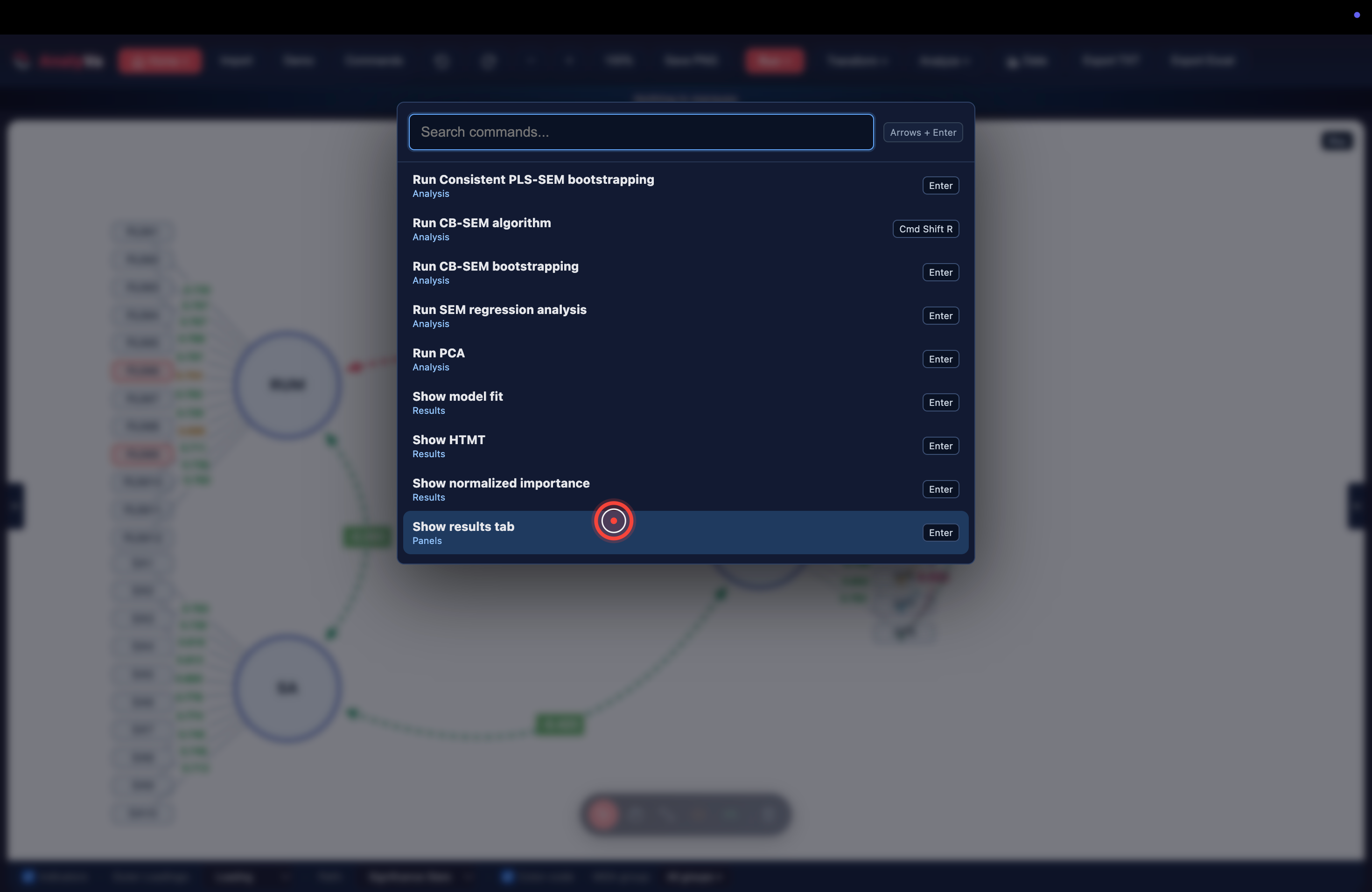
  <li><strong>Show normalized importance</strong> — jumps to IPMA results.</li>
</ul>

<p>If you already ran an analysis, use these to navigate its output
without scrolling.</p>

<h3 id="3-canvas--panels--move-around-the-model">3. Canvas &amp; panels — move around the model</h3>

<p><img src="/blog/images/analyva-shortcuts-03.png" alt="The palette scrolled to canvas commands (Hand tool, Path tool, Zoom in/out, Fit model to view)" /></p>

<p>The bottom of the palette is spatial: tools that manipulate what you
see on the canvas.</p>

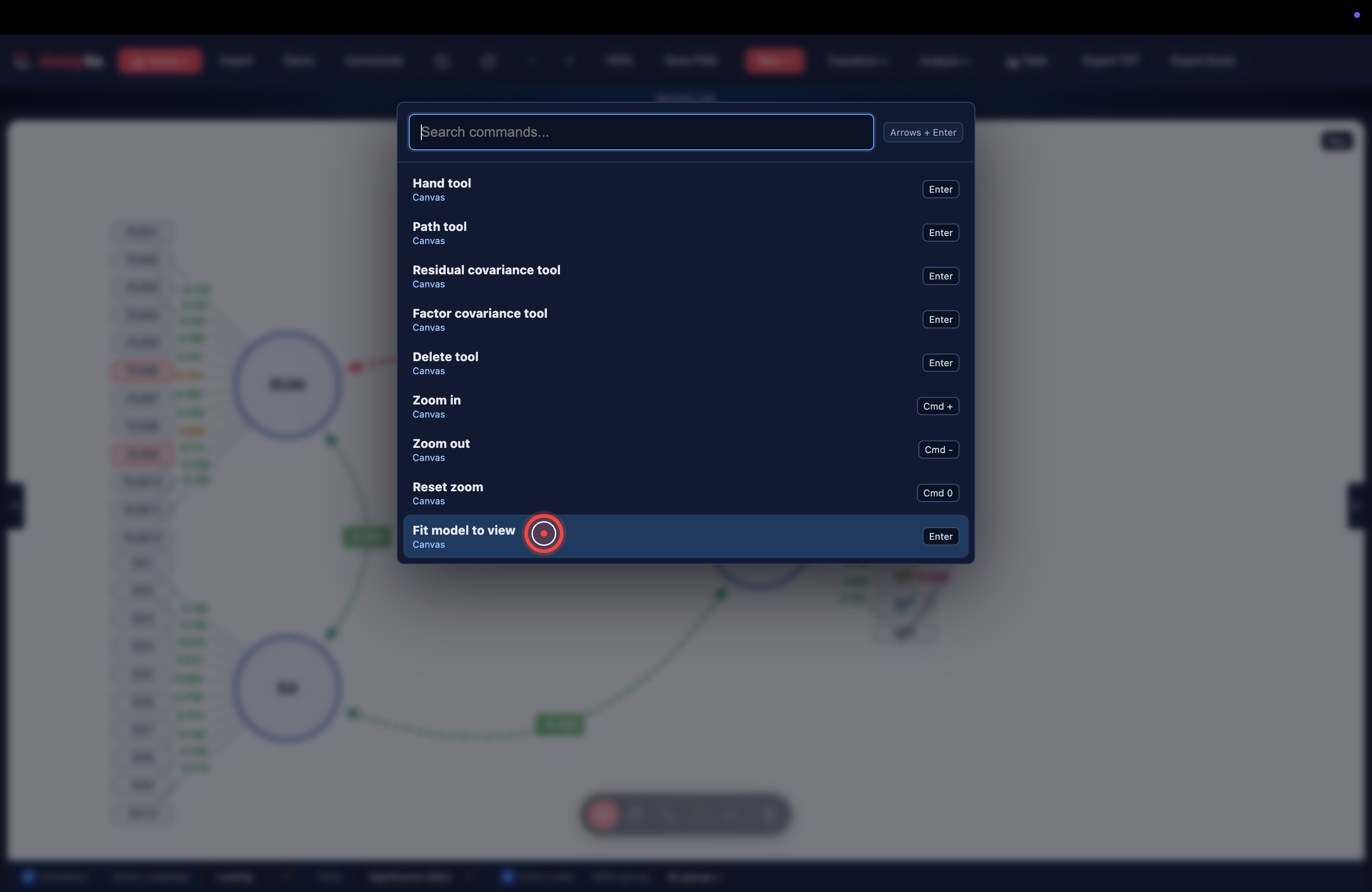
<ul>
  <li><strong>Hand tool</strong> / <strong>Path tool</strong> — switch tool modes without going to
the bottom floating toolbar.</li>
  <li><strong>Residual covariance tool</strong> / <strong>Factor covariance tool</strong> — draw
those two special path types for CB-SEM identification tricks.</li>
  <li><strong>Delete tool</strong> — delete constructs, indicators, or paths.</li>
  <li><strong>Zoom in</strong> / <strong>Zoom out</strong> / <strong>Reset zoom</strong> — <code class="language-plaintext highlighter-rouge">⌘ +</code> / <code class="language-plaintext highlighter-rouge">⌘ -</code> /
<code class="language-plaintext highlighter-rouge">⌘ 0</code>. Same conventions as your browser.</li>
  <li><strong>Fit model to view</strong> — the single most useful spatial command. If
your model has drifted off-screen or you are lost in a big canvas,
this button reframes everything to fit. Add it to muscle memory.</li>
</ul>

<h2 id="the-productivity-pattern">The productivity pattern</h2>

<p>The palette is faster than menus for four specific reasons:</p>

<ol>
  <li><strong>It is search-first, not location-first.</strong> You do not have to
remember which menu contains which command.</li>
  <li><strong>Every command lives there</strong> — including ones that appear only
inside submenus of submenus.</li>
  <li><strong>The keyboard shortcuts are printed on the right</strong> of each row,
so the palette doubles as a discovery mechanism for the shortcuts
themselves.</li>
  <li><strong>The order is stable.</strong> Recently-used commands do not shuffle to
the top, so you build muscle memory for the exact position of
your most-used commands.</li>
</ol>

<h2 id="the-five-shortcuts-to-memorise-this-week">The five shortcuts to memorise this week</h2>

<p>If you only remember five, remember these — they cover roughly 80% of
routine AnalyVa work:</p>

<table>
  <thead>
    <tr>
      <th>Shortcut</th>
      <th>Action</th>
    </tr>
  </thead>
  <tbody>
    <tr>
      <td><code class="language-plaintext highlighter-rouge">⌘ K</code></td>
      <td>Open the command palette</td>
    </tr>
    <tr>
      <td><code class="language-plaintext highlighter-rouge">⌘ I</code></td>
      <td>Import data</td>
    </tr>
    <tr>
      <td><code class="language-plaintext highlighter-rouge">⌘ R</code></td>
      <td>Run PLS-SEM algorithm</td>
    </tr>
    <tr>
      <td><code class="language-plaintext highlighter-rouge">⌘ 0</code></td>
      <td>Reset zoom / <strong>Fit model to view</strong></td>
    </tr>
    <tr>
      <td><code class="language-plaintext highlighter-rouge">⌘ S</code></td>
      <td>Save workspace</td>
    </tr>
  </tbody>
</table>

<p>Do the reps for a week and you will stop reaching for the top menu bar
almost entirely.</p>]]></content><author><name>Abdelouahd Bouzar</name><email>support@analyva.com</email></author><category term="Workflow" /><category term="analyva" /><category term="shortcuts" /><category term="workflow" /><summary type="html"><![CDATA[Skip the menu-diving. Every AnalyVa command — import, run PLS-SEM, show HTMT, switch tools, zoom — is one keystroke away in the command palette.]]></summary><media:thumbnail xmlns:media="http://search.yahoo.com/mrss/" url="https://analyva.com/blog/images/cover-shortcuts.svg" /><media:content medium="image" url="https://analyva.com/blog/images/cover-shortcuts.svg" xmlns:media="http://search.yahoo.com/mrss/" /></entry><entry><title type="html">P-values: What They Actually Mean (and Don’t)</title><link href="https://analyva.com/blog/p-values-what-they-actually-mean/" rel="alternate" type="text/html" title="P-values: What They Actually Mean (and Don’t)" /><published>2026-07-25T00:00:00+00:00</published><updated>2026-07-25T00:00:00+00:00</updated><id>https://analyva.com/blog/p-values-what-they-actually-mean</id><content type="html" xml:base="https://analyva.com/blog/p-values-what-they-actually-mean/"><![CDATA[<p>If you have read a paper in the last twenty years, you have read a
p-value. If you have written one, you have almost certainly reported a
few. And yet — in surveys of researchers, more than 80% define the
p-value incorrectly on the first try. That includes people who use them
every week.</p>

<p>This post is the short, honest version.</p>

<h2 id="what-a-p-value-literally-is">What a p-value literally is</h2>

<p>Formally: <strong>the probability of observing data as extreme as (or more
extreme than) the data you actually observed, assuming the null
hypothesis is true.</strong></p>

<p>In plainer language: “<em>if there were no effect in reality, how surprised
should we be by our results?</em>” A small p-value means “very surprised.”
A large p-value means “not really surprised.”</p>

<p>Notice what a p-value is <em>not</em>. It is not:</p>

<ul>
  <li>the probability that the null hypothesis is true;</li>
  <li>the probability that your finding is a false positive;</li>
  <li>the size of the effect;</li>
  <li>how important the finding is;</li>
  <li>evidence for the alternative hypothesis in any strict sense.</li>
</ul>

<p>Any interpretation that starts with “<em>there is only a 3% chance that the
result is due to chance</em>” is technically wrong. The 3% is a statement
about how unusual the data would be <em>if the null were true</em>, not about
how likely the null is.</p>

<h2 id="the-five-misinterpretations-that-keep-appearing">The five misinterpretations that keep appearing</h2>

<ol>
  <li><strong>“p = .04, so we reject the null and accept the alternative.”</strong>
You reject the null. That is not the same as accepting the
alternative. Rejection just means the data is unlikely under H₀. The
alternative might be true; something else might also be true.</li>
  <li><strong>“p = .06, so we found no effect.”</strong>
You found no <em>significant</em> effect at the .05 threshold. The effect
could be real and moderately sized — you simply lack the sample size
to detect it reliably. Report the effect size regardless.</li>
  <li><strong>“p = .001, so the effect is huge.”</strong>
p-values shrink with sample size. A tiny effect in a study of
100,000 people can produce p &lt; .001 while being practically
meaningless. Always report and interpret an effect size (Cohen’s <em>d</em>,
<em>r</em>, η², <em>f</em>²).</li>
  <li><strong>“Two studies with p = .049 and p = .051 tell opposite stories.”</strong>
They tell nearly identical stories. The .05 cutoff is a convention,
not a phase transition. Treat the values as continuous.</li>
  <li><strong>“Non-significant p-values prove the null hypothesis.”</strong>
Absence of evidence is not evidence of absence. To argue that an
effect is truly zero, you need an equivalence test, a Bayesian
analysis, or a well-justified prior — not simply p &gt; .05.</li>
</ol>

<h2 id="what-p--05-actually-gives-you">What p &lt; .05 actually gives you</h2>

<p>It gives you a <em>decision rule</em> that, over the long run, controls your
false-positive rate at 5% <em>if</em> all the assumptions of your test hold
(independence, distributional assumptions, no p-hacking, no undisclosed
multiple comparisons).</p>

<p>Notice how many “ifs” are in that sentence. In real published research,
those assumptions are rarely all met — which is why the same p-value
carries very different weight in a preregistered replication study
versus an exploratory analysis with 30 tested hypotheses.</p>

<h2 id="what-to-report-alongside-the-p-value">What to report alongside the p-value</h2>

<p>The <a href="https://doi.org/10.1080/00031305.2016.1154108">ASA’s 2016 statement on p-values</a>
recommends that authors go beyond a bare “p &lt; .05.” A defensible modern
report includes:</p>

<ul>
  <li><strong>The effect size</strong> (Cohen’s <em>d</em>, Pearson’s <em>r</em>, η², or standardised
regression coefficient), with its own interpretation.</li>
  <li><strong>A confidence interval</strong> for the effect — it carries all the
information the p-value carries, plus range.</li>
  <li><strong>The exact p-value</strong>, not just “p &lt; .05.” Report <code class="language-plaintext highlighter-rouge">p = .034</code> rather
than <code class="language-plaintext highlighter-rouge">p &lt; .05</code>.</li>
  <li><strong>A note on the number of tests performed</strong>, and any correction
applied (Bonferroni, Holm, FDR).</li>
</ul>

<h2 id="doing-this-in-analyva">Doing this in AnalyVa</h2>

<p>Every inferential test in AnalyVa reports the exact p-value alongside
the effect size, group descriptives, an assumption check, and — where
relevant — a visualisation. Multiple-comparison corrections are one
click away in the same output panel, so nothing about a p-value gets
reported without its context.</p>

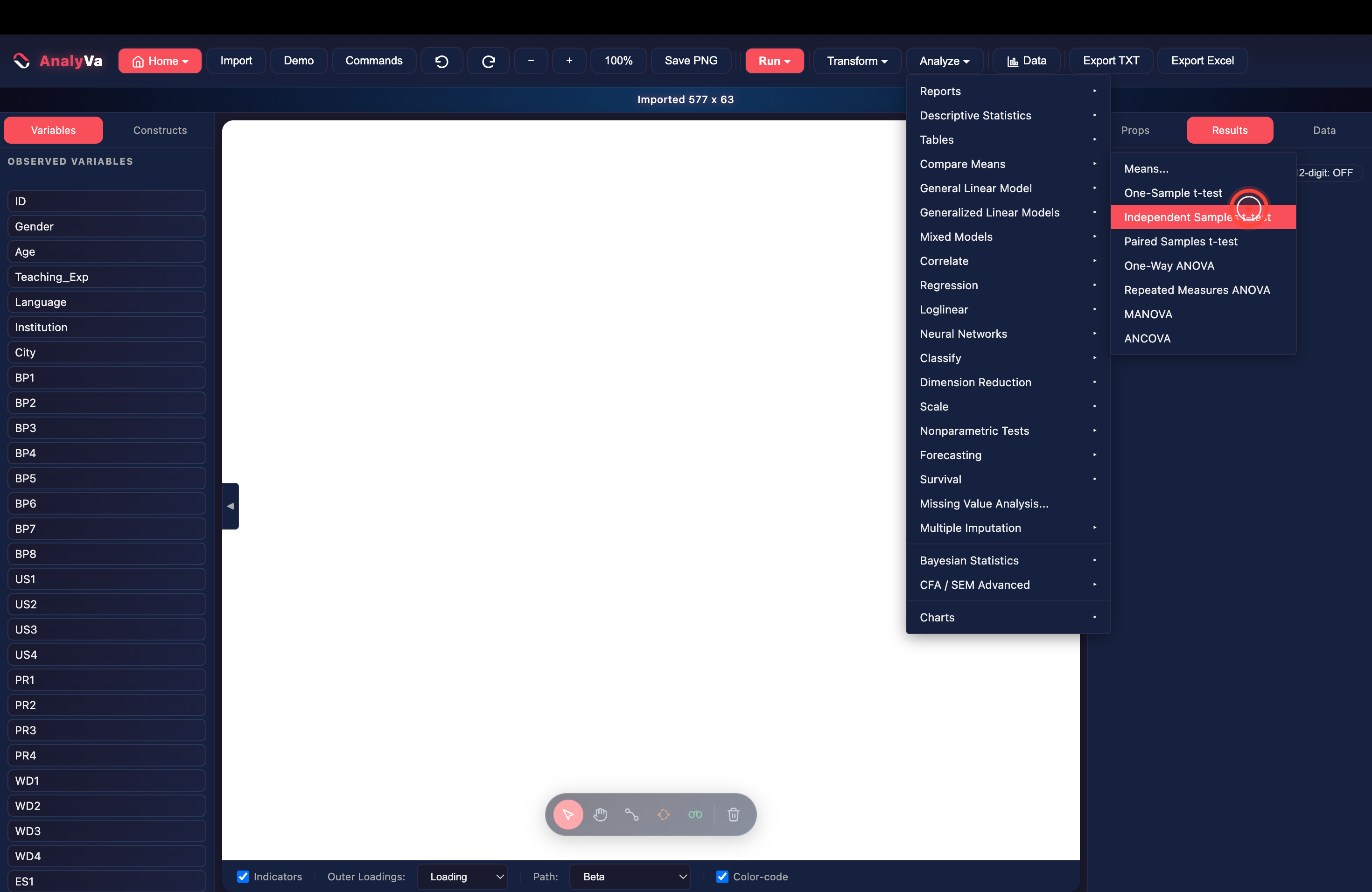
<p>Here is the full workflow, using an independent-samples t-test as the
worked example.</p>

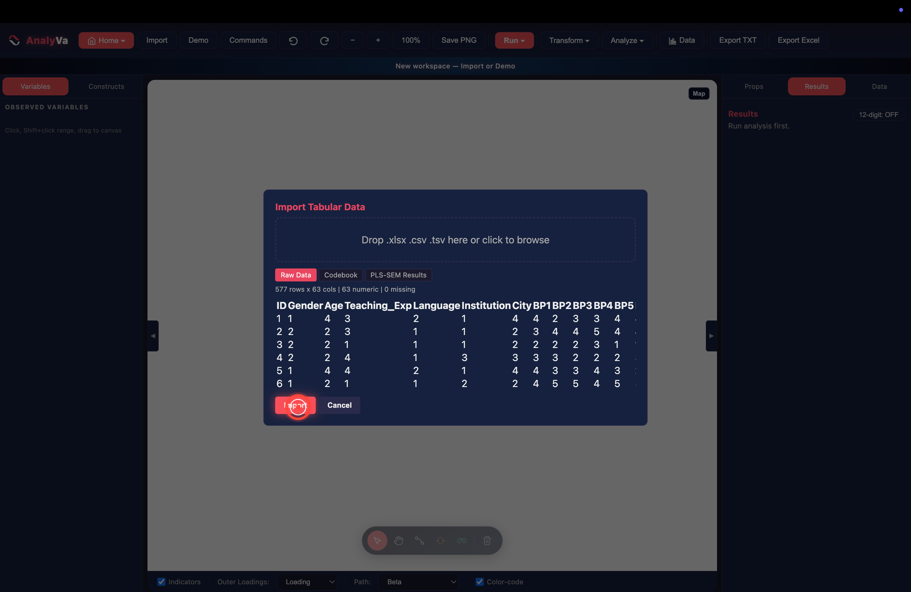
<p><strong>Step 1 — Click <em>Import</em>.</strong>
Launch AnalyVa on an empty canvas. Click the <strong>Import</strong> button in the
top toolbar (second from the left).</p>

<p><img src="/blog/images/analyva-pvalue-01-import-button.png" alt="The Import button in the top toolbar" /></p>

<p><strong>Step 2 — The import dialog opens.</strong>
An overlay appears asking for a file. Accepts <code class="language-plaintext highlighter-rouge">.xlsx</code>, <code class="language-plaintext highlighter-rouge">.csv</code>,
and <code class="language-plaintext highlighter-rouge">.tsv</code>.</p>

<p><img src="/blog/images/analyva-pvalue-02-import-dialog.png" alt="The Import Tabular Data dialog waiting for a file" /></p>

<p><strong>Step 3 — Drop your file and preview.</strong>
Drag your dataset onto the drop zone (or click to browse). AnalyVa
parses it and shows the shape and the first rows for sanity-checking
(here: 577 rows × 63 columns, all numeric, no missing values). Click
<strong>Import</strong> when the preview looks right.</p>

<p><img src="/blog/images/analyva-pvalue-03-import-preview.png" alt="The Import dialog showing a preview of 577 rows × 63 columns" /></p>

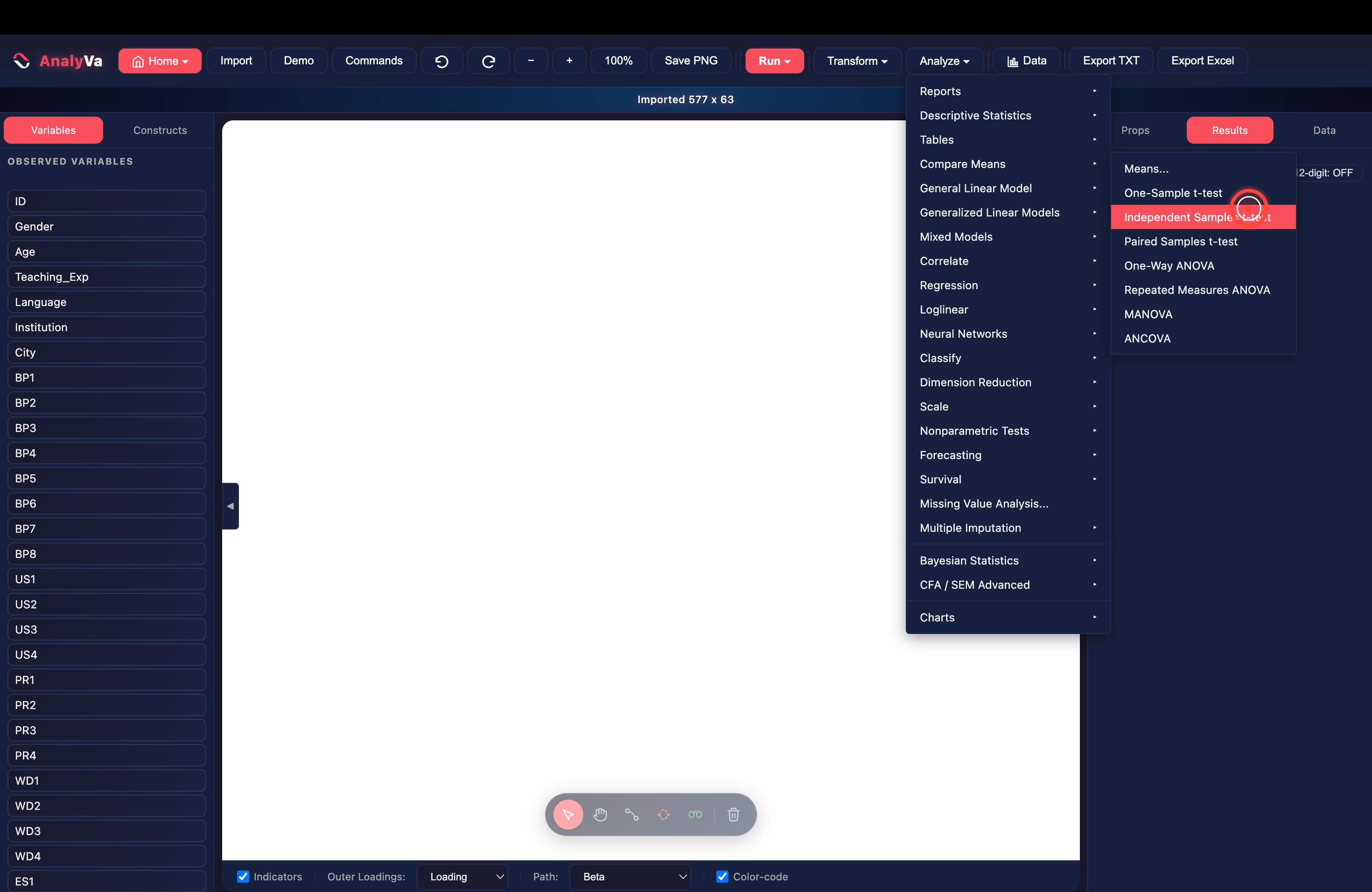
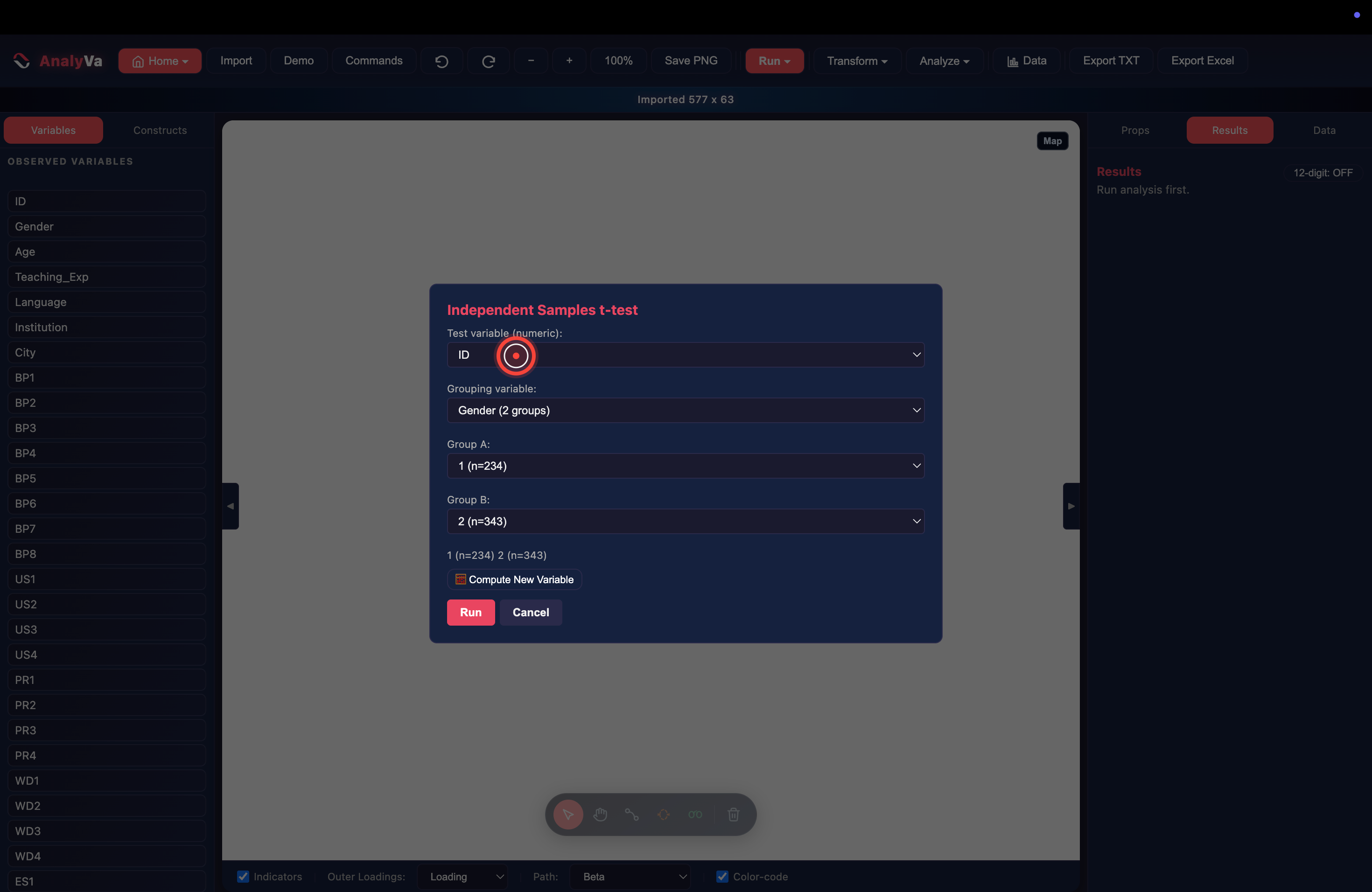
<p><strong>Step 4 — Open <em>Analyze → Compare Means → Independent Samples t-test</em>.</strong>
Every variable in the dataset now appears in the left sidebar. Open
the <strong>Analyze</strong> menu → <strong>Compare Means</strong> → <strong>Independent Samples t-test</strong>.</p>

<p><img src="/blog/images/analyva-pvalue-04-analyze-menu.png" alt="The Analyze menu with Compare Means → Independent Samples t-test highlighted" /></p>

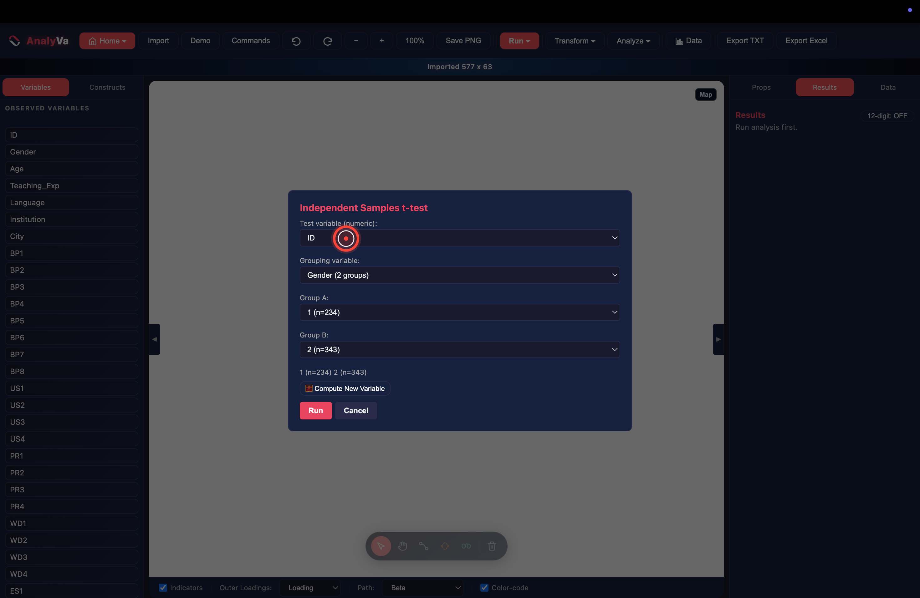
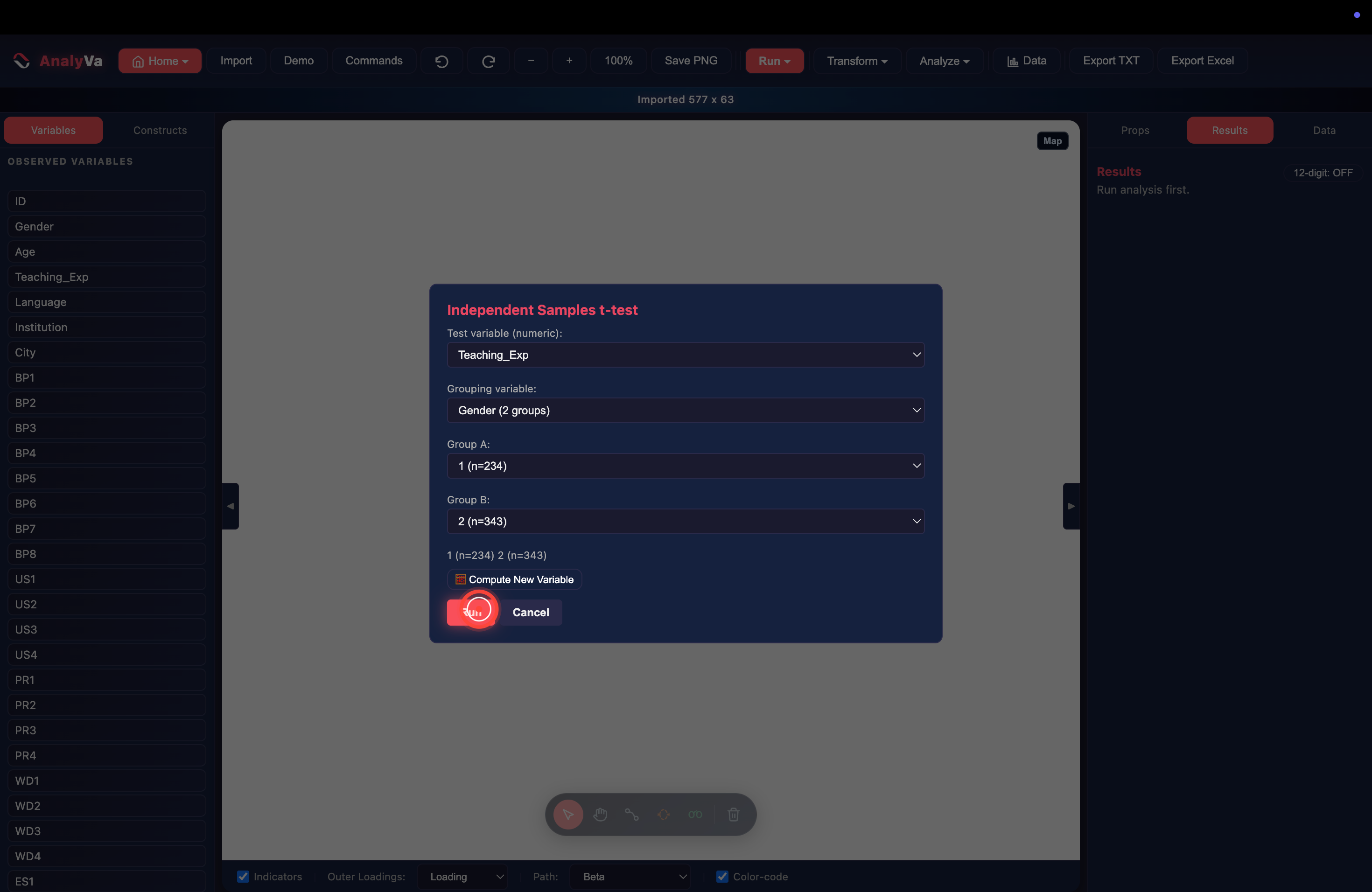
<p><strong>Step 5 — The t-test dialog opens.</strong>
A dialog appears with sensible defaults filled in. AnalyVa
auto-detects the grouping variable and its levels — here Gender has
two groups, Group A = 1 (n = 234), Group B = 2 (n = 343).</p>

<p><img src="/blog/images/analyva-pvalue-05-ttest-dialog.png" alt="The Independent Samples t-test dialog with grouping variable auto-detected" /></p>

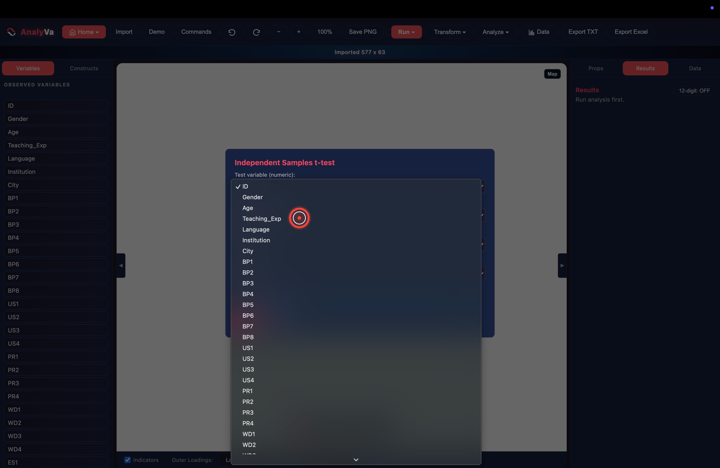
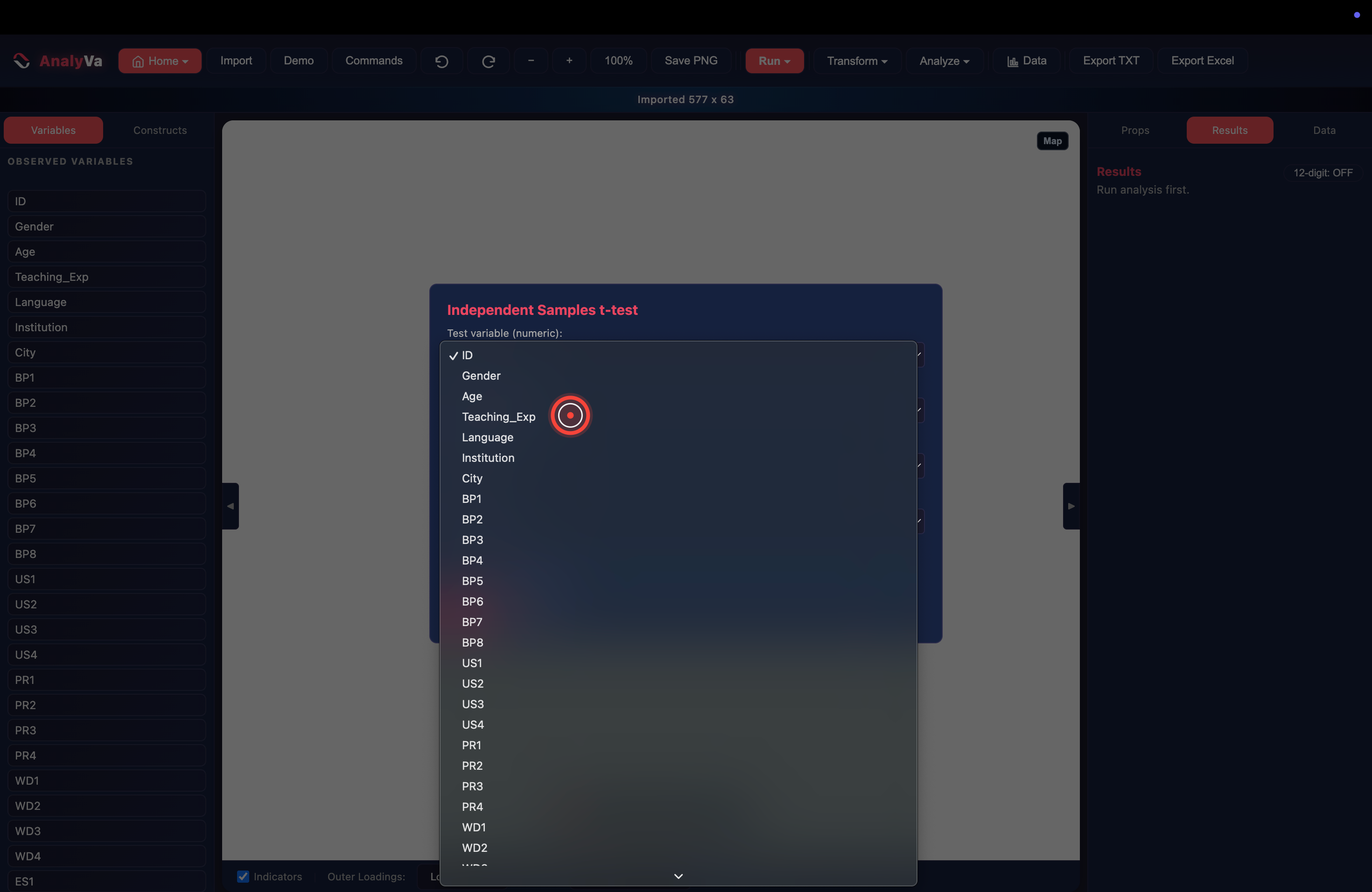
<p><strong>Step 6 — Choose the test variable.</strong>
Open the <em>Test variable</em> dropdown and pick the numeric variable you
want to compare across the two groups. In this example: <code class="language-plaintext highlighter-rouge">Teaching_Exp</code>.</p>

<p><img src="/blog/images/analyva-pvalue-06-select-variable.png" alt="The Test variable dropdown open with Teaching_Exp highlighted" /></p>

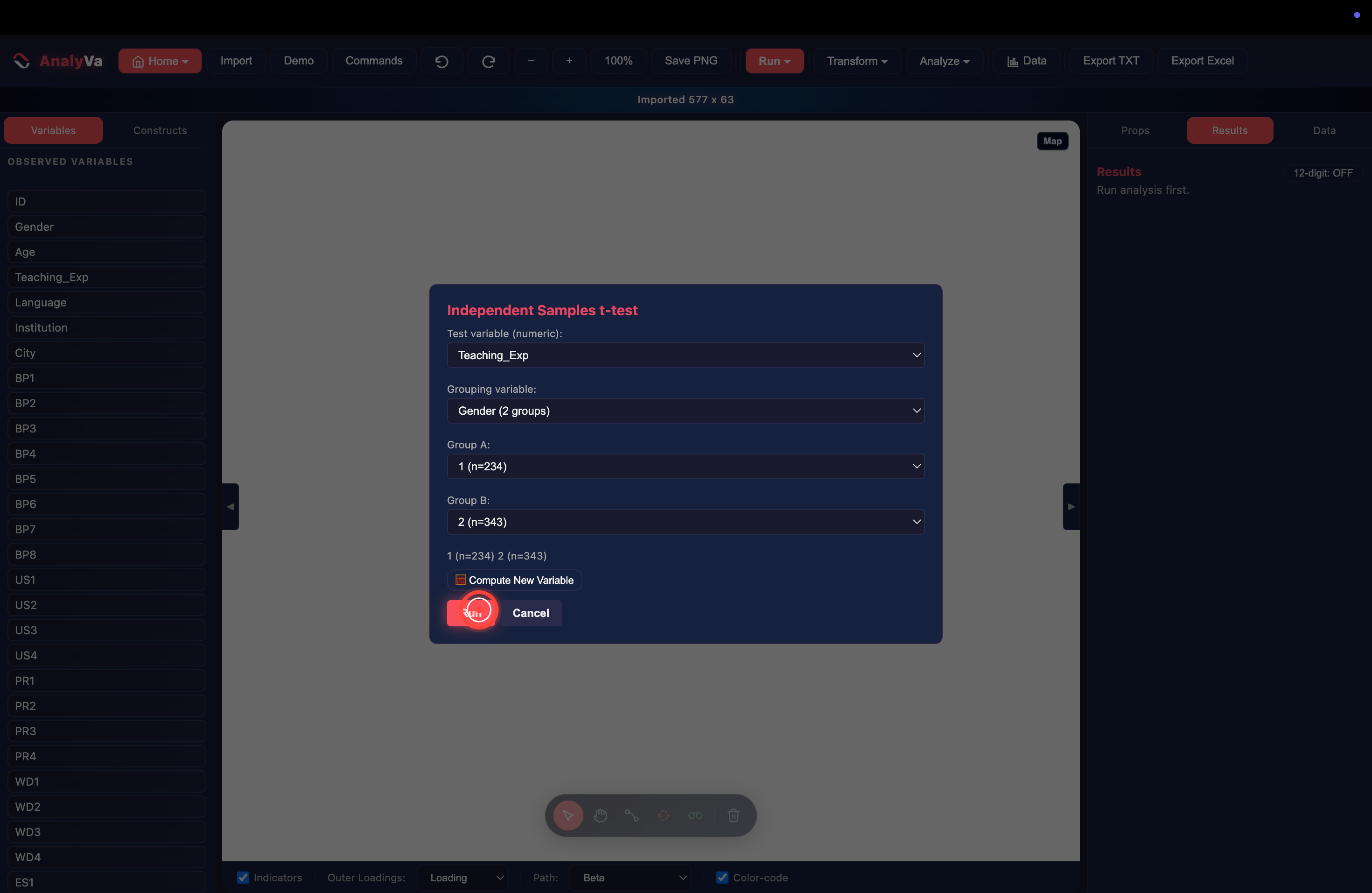
<p><strong>Step 7 — Click <em>Run</em>.</strong>
The dialog now shows your chosen test variable, grouping variable, and
both group sizes. Click the red <strong>Run</strong> button.</p>

<p><img src="/blog/images/analyva-pvalue-07-ready-run.png" alt="The t-test dialog with Teaching_Exp selected and the Run button highlighted" /></p>

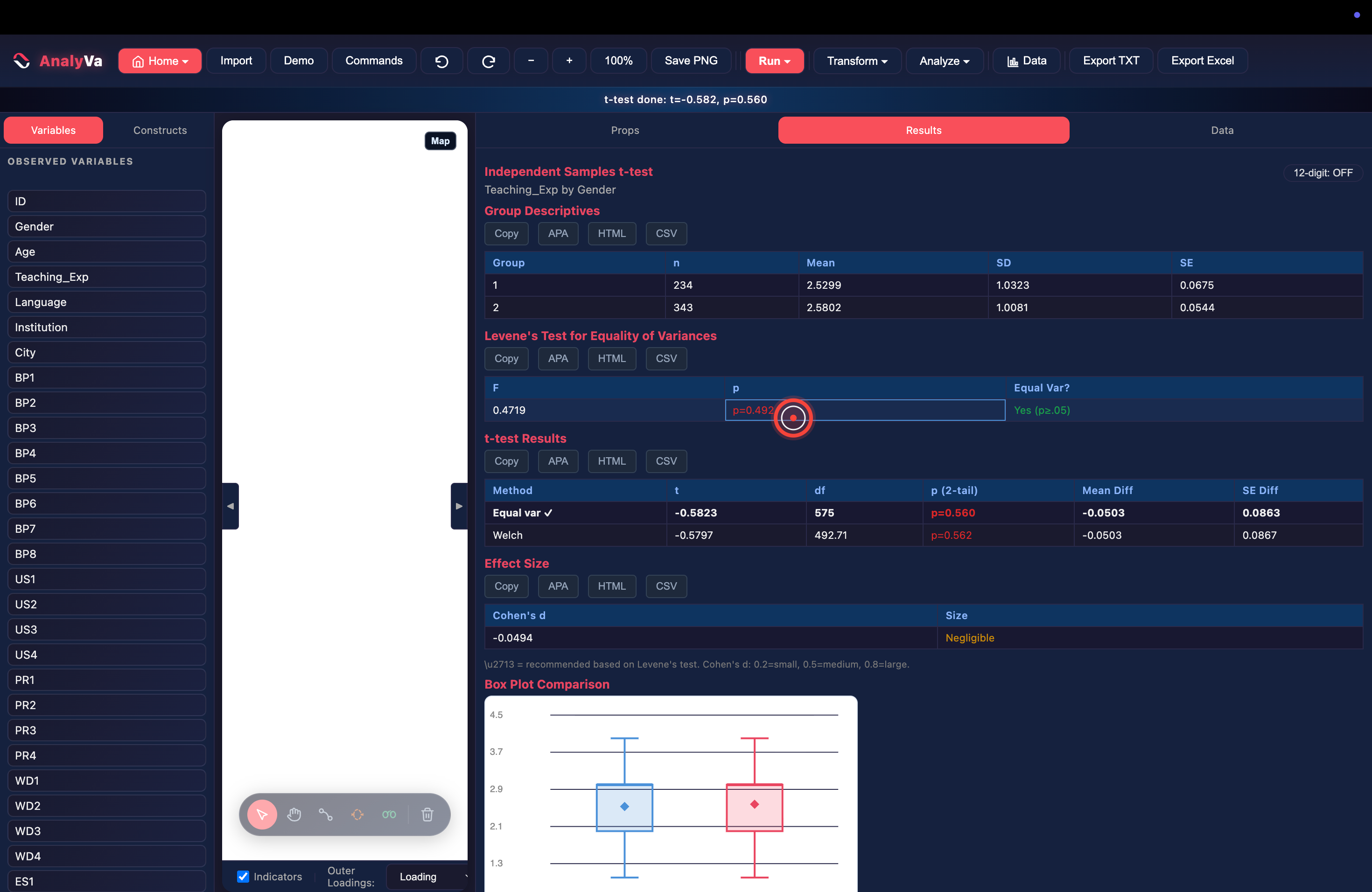
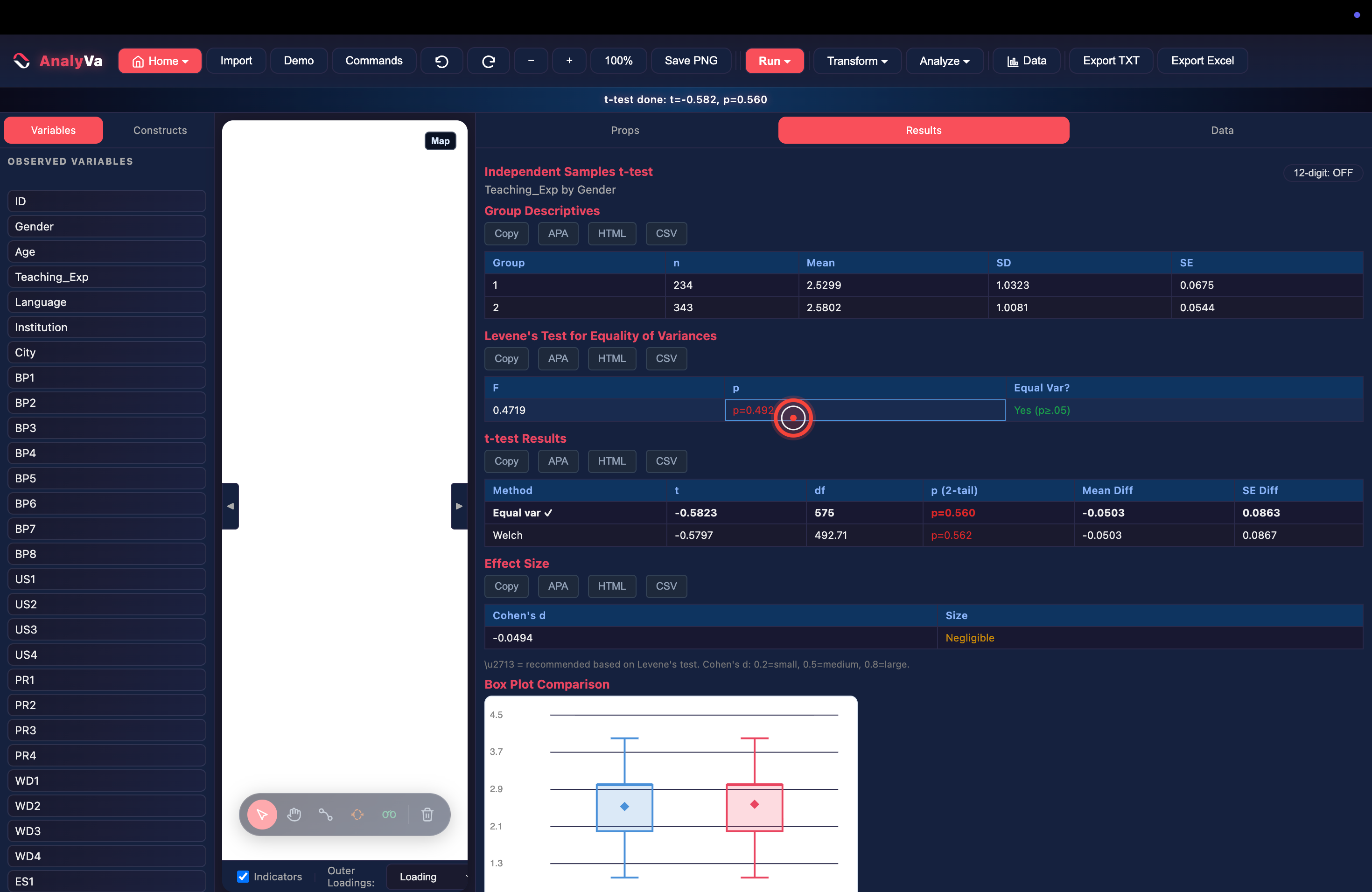
<p><strong>Step 8 — Read the results panel.</strong>
The right pane switches to <strong>Results</strong> and shows every reporting
component in one view:</p>

<ul>
  <li><strong>Group Descriptives</strong> — n, mean, SD, SE per group.</li>
  <li><strong>Levene’s Test for Equality of Variances</strong> — F, p, and a plain-English “Equal Var?” verdict (here: Yes, p ≥ 0.05).</li>
  <li><strong>t-test Results</strong> — both the equal-variance version (t = -0.582, df = 575, p = 0.560) <em>and</em> Welch’s (t = -0.580, df = 492.71, p = 0.562), with a checkmark on the one Levene recommends.</li>
  <li><strong>Effect Size</strong> — Cohen’s d = -0.049, labelled <em>Negligible</em>.</li>
  <li><strong>Box Plot Comparison</strong> — a side-by-side visualisation.</li>
</ul>

<p>Notice how the interpretation lives right next to the p-value. You
never have to hunt for the effect size, the assumption check, or the
alternative test — everything a defensible report needs is in one
scroll.</p>

<p><img src="/blog/images/analyva-pvalue-08-results.png" alt="Independent Samples t-test results panel showing group descriptives, Levene, t-test values, Cohen's d, and a box plot" /></p>

<p>Every table has its own <strong>Copy</strong>, <strong>APA</strong>, <strong>HTML</strong>, and <strong>CSV</strong> button
above it — so a properly formatted APA sentence
(<em>“t(575) = -0.58, p = .560, d = -0.05”</em>) is one click away.</p>

<h2 id="further-reading">Further reading</h2>

<ul>
  <li>Wasserstein, R. L., &amp; Lazar, N. A. (2016). The ASA’s statement on
p-values: Context, process, and purpose. <em>The American Statistician</em>,
70(2), 129–133. <a href="https://doi.org/10.1080/00031305.2016.1154108">DOI</a></li>
  <li>Amrhein, V., Greenland, S., &amp; McShane, B. (2019). Scientists rise up
against statistical significance. <em>Nature</em>, 567, 305–307.</li>
</ul>]]></content><author><name>Abdelouahd Bouzar</name><email>support@analyva.com</email></author><category term="Statistics" /><category term="statistics" /><category term="p-value" /><category term="hypothesis testing" /><summary type="html"><![CDATA[What does a p-value actually mean? The formal definition in plain language, the five misinterpretations that appear in peer-reviewed papers, and what to report alongside it.]]></summary><media:thumbnail xmlns:media="http://search.yahoo.com/mrss/" url="https://analyva.com/blog/images/cover-p-value.jpg" /><media:content medium="image" url="https://analyva.com/blog/images/cover-p-value.jpg" xmlns:media="http://search.yahoo.com/mrss/" /></entry><entry><title type="html">HTMT Above 0.85: What to Do When Discriminant Validity Fails</title><link href="https://analyva.com/blog/htmt-above-0-85-what-to-do/" rel="alternate" type="text/html" title="HTMT Above 0.85: What to Do When Discriminant Validity Fails" /><published>2026-07-24T00:00:00+00:00</published><updated>2026-07-24T00:00:00+00:00</updated><id>https://analyva.com/blog/htmt-above-0-85-what-to-do</id><content type="html" xml:base="https://analyva.com/blog/htmt-above-0-85-what-to-do/"><![CDATA[<p>You ran PLS-SEM, opened the report, and one HTMT value is 0.87. The
manuscript is due Friday. The reviewer you’re most worried about wrote
their PhD on discriminant validity. What now?</p>

<p>This post gives you a concrete decision path — the same one used by
methodologists like <a href="https://doi.org/10.1007/s11747-014-0403-8">Henseler, Ringle, and Sarstedt (2015)</a> and
extended in later work. It applies whether you’re running the analysis
in SmartPLS 4, in R with the <code class="language-plaintext highlighter-rouge">SEMinR</code> or <code class="language-plaintext highlighter-rouge">cSEM</code> packages, or in AnalyVa.</p>

<h2 id="what-htmt-actually-measures">What HTMT actually measures</h2>

<p>The <strong>Heterotrait-Monotrait ratio of correlations (HTMT)</strong> compares the
average correlation of indicators <em>across</em> two constructs to the average
correlation of indicators <em>within</em> each construct. When HTMT approaches
1.0, the two constructs are effectively measuring the same thing.</p>

<p>There isn’t one universally accepted cutoff. The three most commonly
cited thresholds are:</p>

<ul>
  <li><strong>HTMT &lt; 0.85</strong> — strict. Recommended when your constructs are
conceptually distinct (e.g., <em>trust</em> vs. <em>satisfaction</em>).</li>
  <li><strong>HTMT &lt; 0.90</strong> — liberal. Acceptable when constructs are
conceptually close (e.g., <em>cognitive trust</em> vs. <em>affective trust</em>).</li>
  <li><strong>HTMT confidence interval excludes 1.0</strong> — the inferential test,
based on bootstrap resampling. Preferred by many editors today.</li>
</ul>

<p>If your value sits between 0.85 and 0.90, don’t panic yet — the
inferential HTMT test is what most journals now expect you to report
anyway.</p>

<h2 id="the-six-things-to-try-in-order">The six things to try, in order</h2>

<h3 id="1-check-the-bootstrapped-htmt-confidence-interval">1. Check the bootstrapped HTMT confidence interval</h3>

<p>Run 5,000 bootstrap subsamples with the percentile method and report
the 97.5% upper bound. If the interval excludes 1.0, most reviewers
will accept the constructs as empirically distinct even when the point
estimate is above 0.85. This is the test that survives peer review.</p>

<h3 id="2-look-at-the-offending-indicator-pair">2. Look at the offending indicator pair</h3>

<p>HTMT is an <em>average</em> — it hides which specific pair is causing the
problem. Pull the raw cross-loadings matrix and find the two indicators
with the highest cross-construct correlation. That pair is usually
where the theoretical overlap is real.</p>

<h3 id="3-consider-whether-the-constructs-are-actually-distinct">3. Consider whether the constructs are actually distinct</h3>

<p>Sometimes HTMT is telling you the truth: the two constructs <em>aren’t</em>
distinct in your data. This is the moment to step back from the
statistics and ask a theoretical question. Are <em>perceived usefulness</em>
and <em>perceived value</em> really separate for your sample, or did your
respondents treat them as the same idea? If the constructs collapse
conceptually, merge them and reestimate.</p>

<h3 id="4-drop-the-weakest-cross-loading-indicator">4. Drop the weakest cross-loading indicator</h3>

<p>If the pair problem is driven by one indicator with a weak outer
loading (&lt; 0.70) and a strong cross-loading, drop it. Document the
decision in the methods section. Never drop indicators purely to
“fix” HTMT — you need a defensible measurement reason.</p>

<h3 id="5-reconsider-the-reflectiveformative-specification">5. Reconsider the reflective/formative specification</h3>

<p>If one of the constructs is actually formative (its indicators <em>cause</em>
the latent variable rather than reflect it), HTMT doesn’t apply in the
first place. Formative constructs are assessed with VIF and indicator
weights, not with HTMT or AVE. Misspecification is a common hidden
cause of “failing” discriminant validity.</p>

<h3 id="6-if-all-else-fails-report-and-defend">6. If all else fails, report and defend</h3>

<p>If the theory supports two distinct constructs, the bootstrapped HTMT
interval excludes 1.0, and dropping indicators would harm construct
coverage, report the HTMT value honestly and defend it in the
Discussion. Editors generally accept a defended 0.87 more readily than
a suspiciously clean 0.84 that clearly came from indicator surgery.</p>

<h2 id="how-this-looks-in-smartpls-4">How this looks in SmartPLS 4</h2>

<p>SmartPLS 4 reports the HTMT point estimate in the standard PLS
algorithm output, and the bootstrapped confidence intervals under the
“Discriminant Validity” tab after you run the bootstrap procedure. To
identify the offending indicator pair, open the “Cross Loadings”
report.</p>

<h2 id="doing-this-in-analyva">Doing this in AnalyVa</h2>

<p>The full workflow, from a fresh canvas to an HTMT verdict on every
construct pair in the model.</p>

<p><strong>Step 1 — Click <em>Import</em>.</strong>
Launch AnalyVa on an empty canvas. Click the <strong>Import</strong> button in the
top toolbar.</p>

<p><img src="/blog/images/analyva-htmt-01-import-button.png" alt="The Import button in the top toolbar" /></p>

<p><strong>Step 2 — The import dialog opens.</strong>
An overlay appears asking for a file (<code class="language-plaintext highlighter-rouge">.xlsx</code>, <code class="language-plaintext highlighter-rouge">.csv</code>, or <code class="language-plaintext highlighter-rouge">.tsv</code>).</p>

<p><img src="/blog/images/analyva-htmt-02-import-dialog.png" alt="The Import Tabular Data dialog waiting for a file" /></p>

<p><strong>Step 3 — Load the file and preview it.</strong>
Drop your dataset. AnalyVa parses it and reports the shape (here:
1,311 rows × 49 columns, all numeric, no missing). The first six rows
appear so you can sanity-check. Click <strong>Import</strong>.</p>

<p><img src="/blog/images/analyva-htmt-03-import-preview.png" alt="The Import dialog showing the file preview and the Import button" /></p>

<p><strong>Step 4 — Build the first construct.</strong>
Every variable now appears in the sidebar. To create a construct,
click its first indicator in the sidebar (here, <code class="language-plaintext highlighter-rouge">C1</code>).</p>

<p><img src="/blog/images/analyva-htmt-04-select-c-first.png" alt="The sidebar with C1 selected" /></p>

<p><strong>Step 5 — Shift-click the last indicator to select the range.</strong>
Shift-click <code class="language-plaintext highlighter-rouge">C7</code> (or Ctrl/Cmd-click individual items). The sidebar
highlights the whole range in red. Then drag the selection onto the
canvas — AnalyVa creates a construct named after the item prefix
(here: <code class="language-plaintext highlighter-rouge">C</code>) with all 7 indicators attached.</p>

<p><img src="/blog/images/analyva-htmt-05-select-c-all.png" alt="All 7 C items highlighted in the sidebar" /></p>

<p><strong>Step 6 — Repeat for the second construct.</strong>
The canvas now shows two constructs (<code class="language-plaintext highlighter-rouge">C</code> and <code class="language-plaintext highlighter-rouge">DP</code> — DP was created the
same way earlier). To add the third, click the first indicator of the
new construct in the sidebar (here: <code class="language-plaintext highlighter-rouge">MC1</code>).</p>

<p><img src="/blog/images/analyva-htmt-06-select-mc-first.png" alt="MC1 selected in the sidebar" /></p>

<p><strong>Step 7 — Shift-click through the range.</strong>
Shift-click <code class="language-plaintext highlighter-rouge">MC6</code> to select all six MC items.</p>

<p><img src="/blog/images/analyva-htmt-07-select-mc-range.png" alt="MC1–MC5 highlighted, cursor on MC6" /></p>

<p><strong>Step 8 — All six items selected.</strong>
The MC block is now fully highlighted in the sidebar.</p>

<p><img src="/blog/images/analyva-htmt-08-select-mc-all.png" alt="All 6 MC items highlighted" /></p>

<p><strong>Step 9 — Drop the MC construct onto the canvas.</strong>
Drag the highlighted MC items onto the canvas. AnalyVa creates the
<code class="language-plaintext highlighter-rouge">MC</code> construct with all 6 indicators. Click the new construct — the
right pane switches to <strong>Props</strong> and shows its type (<code class="language-plaintext highlighter-rouge">reflective</code>) and
indicator list.</p>

<p><img src="/blog/images/analyva-htmt-09-mc-construct.png" alt="The MC construct on the canvas with its Props panel visible" /></p>

<p><strong>Step 10 — Switch to the Path tool.</strong>
At the bottom of the canvas is a small floating toolbar. The second
button from the left is the <strong>Path (P)</strong> tool — click it (or press
<code class="language-plaintext highlighter-rouge">P</code>).</p>

<p><img src="/blog/images/analyva-htmt-10-path-tool.png" alt="The Path tool in the floating toolbar" /></p>

<p><strong>Step 11 — Start drawing a path.</strong>
With the Path tool active, click the source construct. The cursor is
now attached to that construct.</p>

<p><img src="/blog/images/analyva-htmt-11-path-drawing.png" alt="Path tool active, cursor on the DP construct" /></p>

<p><strong>Step 12 — Draw H1: DP → MC.</strong>
Click the target construct to complete the path. AnalyVa auto-labels
it <code class="language-plaintext highlighter-rouge">H1</code> and displays the hypothesis in the header bar (<em>“H1: Path: DP
-&gt; MC”</em>).</p>

<p><img src="/blog/images/analyva-htmt-12-path-h1.png" alt="The first path H1 drawn from DP to MC" /></p>

<p><strong>Step 13 — Draw H2: C → MC.</strong>
Click C, then click MC. Path H2 is drawn.</p>

<p><img src="/blog/images/analyva-htmt-13-path-h2.png" alt="H1 and H2 paths on the canvas" /></p>

<p><strong>Step 14 — Draw H3: DP → C.</strong>
Click DP, then click C. All three hypothesis paths are now drawn. The
header confirms <em>“H3: Path: DP -&gt; C”</em>.</p>

<p><img src="/blog/images/analyva-htmt-14-path-h3.png" alt="All three paths drawn — H1, H2, H3" /></p>

<p><strong>Step 15 — Open <em>Run → PLS-SEM → Standard Algorithms → PLS-SEM
algorithm</em>.</strong>
The model is ready to estimate. Open the <strong>Run</strong> menu → <strong>PLS-SEM</strong> →
<strong>Standard Algorithms</strong> → <strong>PLS-SEM algorithm</strong>.</p>

<p><img src="/blog/images/analyva-htmt-15-run-menu.png" alt="The Run menu with PLS-SEM → Standard Algorithms → PLS-SEM algorithm" /></p>

<p><strong>Step 16 — Configure and <em>Start calculation</em>.</strong>
A configuration dialog opens: weighting scheme (Factor / Path / PCA),
initial weights, missing-value handling. The defaults are the
Hair et al. recommendations (Path weighting, mean replacement) and
AnalyVa also reports the current data profile — 1,311 rows, 28,842
indicator cells, 0 missing. Leave the defaults and click <strong>Start
calculation</strong>.</p>

<p><img src="/blog/images/analyva-htmt-16-pls-config.png" alt="The PLS-SEM algorithm configuration dialog with Start calculation highlighted" /></p>

<p><strong>Step 17 — Read the HTMT table.</strong>
The right pane switches to <strong>Results</strong> and streams every report the
Hair et al. checklist requires. The <strong>HTMT</strong> table sits high on the
page with the verdict already labelled:</p>

<ul>
  <li><strong>DP – C:</strong> 0.4180 → <em>Good</em></li>
  <li><strong>DP – MC:</strong> 0.4821 → <em>Good</em></li>
  <li><strong>C – MC:</strong> 0.7090 → <em>Good</em></li>
</ul>

<p>All three pairs are safely below 0.85. Outer VIF, Fornell-Larcker,
cross-loadings, and the path diagram with computed loadings (0.827,
0.791, …) and path coefficients (0.384, 0.555, 0.228) are all
generated in the same run — nothing to re-execute.</p>

<p>If any HTMT pair here had exceeded 0.85, the workflow to fix it starts
right back at the top of this post: check the bootstrap CI, find the
offending indicator pair in the cross-loadings table below, and
decide.</p>

<p><img src="/blog/images/analyva-htmt-17-htmt-results.png" alt="The Results panel showing the HTMT table with all three construct pairs marked Good" /></p>

<h2 id="validation">Validation</h2>

<p>AnalyVa’s HTMT calculations were benchmarked against SmartPLS 4 on the
corporate reputation dataset (n = 344) as part of the second
validation study. Point estimates and bootstrapped confidence intervals
reproduce SmartPLS output to the reported precision. See the study on
Zenodo at <a href="https://doi.org/10.5281/zenodo.21536948">doi.org/10.5281/zenodo.21536948</a>.</p>

<h2 id="further-reading">Further reading</h2>

<ul>
  <li>Henseler, J., Ringle, C. M., &amp; Sarstedt, M. (2015). A new criterion
for assessing discriminant validity in variance-based structural
equation modeling. <em>Journal of the Academy of Marketing Science</em>,
43(1), 115–135. <a href="https://doi.org/10.1007/s11747-014-0403-8">DOI</a></li>
  <li>Franke, G., &amp; Sarstedt, M. (2019). Heuristics versus statistics in
discriminant validity testing. <em>Internet Research</em>, 29(3), 430–447.</li>
</ul>]]></content><author><name>Abdelouahd Bouzar</name><email>support@analyva.com</email></author><category term="PLS-SEM" /><category term="PLS-SEM" /><category term="HTMT" /><category term="discriminant validity" /><summary type="html"><![CDATA[HTMT crossed 0.85 in your PLS-SEM report? A step-by-step decision path: check the bootstrap CI, inspect indicator pairs, and defend or reshape the model.]]></summary><media:thumbnail xmlns:media="http://search.yahoo.com/mrss/" url="https://analyva.com/blog/images/cover-htmt.jpg" /><media:content medium="image" url="https://analyva.com/blog/images/cover-htmt.jpg" xmlns:media="http://search.yahoo.com/mrss/" /></entry><entry><title type="html">T-Tests: When to Use Which</title><link href="https://analyva.com/blog/t-tests-when-to-use-which/" rel="alternate" type="text/html" title="T-Tests: When to Use Which" /><published>2026-07-23T00:00:00+00:00</published><updated>2026-07-23T00:00:00+00:00</updated><id>https://analyva.com/blog/t-tests-when-to-use-which</id><content type="html" xml:base="https://analyva.com/blog/t-tests-when-to-use-which/"><![CDATA[<p>The t-test is the workhorse of comparing means. But “the t-test” is
really <em>three</em> related tests, and picking the wrong one is one of the
most common mistakes in student and early-career research.</p>

<p>Here is the decision framework and the reporting standards.</p>

<h2 id="the-three-t-tests">The three t-tests</h2>

<p><strong>One-sample t-test.</strong>
Compares one group’s mean to a known reference value.
<em>Example: are the students in this sample scoring above the national
average of 100?</em></p>

<p><strong>Independent-samples t-test.</strong>
Compares the means of two <em>different</em> groups.
<em>Example: do men and women differ in exam scores?</em></p>

<p><strong>Paired-samples t-test.</strong>
Compares two measurements from the <em>same</em> subjects (or matched pairs).
<em>Example: did the students’ scores change from pre-test to post-test?</em></p>

<p>Using the wrong one inflates or deflates the Type I error rate. An
independent test on paired data throws away statistical power; a paired
test on independent data is simply invalid.</p>

<h2 id="decision-tree">Decision tree</h2>

<ul>
  <li>Comparing <strong>one group</strong> to a fixed number? → <strong>one-sample.</strong></li>
  <li>Comparing <strong>two independent groups</strong>? → <strong>independent.</strong></li>
  <li>Comparing <strong>two measurements from the same subjects</strong> (or matched
pairs)? → <strong>paired.</strong></li>
  <li>Comparing <strong>three or more groups</strong>? → not a t-test. Use ANOVA.</li>
</ul>

<h2 id="assumptions">Assumptions</h2>

<p>All t-tests assume:</p>

<ul>
  <li>the dependent variable is continuous (interval or ratio);</li>
  <li>observations are independent within each group;</li>
  <li>the dependent variable is approximately normally distributed within
each group.</li>
</ul>

<p>The independent-samples t-test additionally assumes equal variances
between groups (homogeneity). When that is violated, use <strong>Welch’s
t-test</strong> — most modern statistical software defaults to Welch’s for
exactly this reason. It costs nothing when variances are equal and
works correctly when they are not.</p>

<h2 id="effect-size--report-it-always">Effect size — report it, always</h2>

<p>A p-value tells you whether a difference exists. Cohen’s <em>d</em> tells you
how big it is.</p>

<ul>
  <li><strong>d = 0.20</strong> → small</li>
  <li><strong>d = 0.50</strong> → medium</li>
  <li><strong>d = 0.80</strong> → large</li>
</ul>

<p>A study with n = 1,000 might return <code class="language-plaintext highlighter-rouge">p &lt; .001</code> for <code class="language-plaintext highlighter-rouge">d = 0.05</code> —
statistically significant, practically meaningless. Always report d
alongside its 95% confidence interval.</p>

<h2 id="three-common-mistakes">Three common mistakes</h2>

<p><strong>1. Running pairwise t-tests on three or more groups.</strong>
Three groups A, B, C tested with three t-tests (A vs B, A vs C, B vs C),
each at α = 0.05, gives a family-wise error rate of roughly 14%. Use
ANOVA followed by a post-hoc test (Tukey’s HSD, Bonferroni) instead.</p>

<p><strong>2. Ignoring Welch’s t-test.</strong>
When group variances differ notably (Levene’s test p &lt; 0.05), the
classical Student’s t-test is biased. Welch’s has no such assumption.
Modern journals expect Welch’s by default when variances are unequal.</p>

<p><strong>3. One-tailed tests without prior justification.</strong>
A one-tailed test doubles statistical power on one side, but requires
you to have committed to a direction <em>before</em> looking at the data.
Post-hoc one-tailed tests are a form of p-hacking. Report two-tailed by
default unless you have a preregistered directional hypothesis.</p>

<h2 id="what-to-report">What to report</h2>

<p>For an independent-samples t-test, a defensible modern report:</p>

<blockquote>
  <p>“The intervention group scored significantly higher than the control
group, t(48) = 3.21, p = .002, d = 0.91, 95% CI for d [0.34, 1.48].”</p>
</blockquote>

<p>Components:</p>

<ul>
  <li><strong>t(df) = value</strong> — the statistic and its degrees of freedom.</li>
  <li><strong>exact p</strong> — not just “&lt; .05”.</li>
  <li><strong>Cohen’s d</strong> plus its 95% CI.</li>
  <li><strong>The mean difference</strong> plus its 95% CI where journal style allows.</li>
</ul>

<h2 id="doing-this-in-analyva">Doing this in AnalyVa</h2>

<p>The workflow is almost identical for all three t-test variants — the
only real decision point is which one you pick from the menu in
Step 4. This walkthrough uses an <strong>Independent Samples t-test</strong> as the
worked example, and calls out at each step how the other two variants
diverge.</p>

<p><strong>Step 1 — Click <em>Import</em>.</strong>
Launch AnalyVa on an empty canvas. Click the <strong>Import</strong> button in the
top toolbar.</p>

<p><img src="/blog/images/analyva-ttest-01-import-button.png" alt="The Import button in the top toolbar" /></p>

<p><strong>Step 2 — The import dialog opens.</strong>
An overlay appears asking for a file (<code class="language-plaintext highlighter-rouge">.xlsx</code>, <code class="language-plaintext highlighter-rouge">.csv</code>, or <code class="language-plaintext highlighter-rouge">.tsv</code>).</p>

<p><img src="/blog/images/analyva-ttest-02-import-dialog.png" alt="The Import Tabular Data dialog waiting for a file" /></p>

<p><strong>Step 3 — Load and preview.</strong>
Drop your dataset. AnalyVa reports the shape and shows the first rows
so you can confirm it parsed correctly. Click <strong>Import</strong>.</p>

<p>Your dataset needs to include:</p>

<ul>
  <li><strong>One-sample:</strong> the continuous variable of interest;</li>
  <li><strong>Independent-samples:</strong> a continuous outcome + a grouping variable
with exactly two levels;</li>
  <li><strong>Paired-samples:</strong> two continuous variables measured on the same
cases (pre + post, spouse-A + spouse-B, etc.).</li>
</ul>

<p><img src="/blog/images/analyva-ttest-03-import-preview.png" alt="The Import dialog showing a preview of the data" /></p>

<p><strong>Step 4 — Pick the right t-test from <em>Analyze → Compare Means</em>.</strong>
This is the only decision that changes. Open the <strong>Analyze</strong> menu →
<strong>Compare Means</strong>. The submenu lists all three t-tests explicitly:</p>

<ul>
  <li><strong>One-Sample t-test</strong> — for comparing one group’s mean to a fixed
reference value.</li>
  <li><strong>Independent Samples t-test</strong> — for two different groups (this
example).</li>
  <li><strong>Paired Samples t-test</strong> — for two measurements from the same
subjects.</li>
</ul>

<p>If your design matches multiple items, re-read the decision tree
earlier in this post — only one of them is appropriate for any given
research question.</p>

<p><img src="/blog/images/analyva-ttest-04-choose-test-type.png" alt="The Analyze → Compare Means submenu showing all three t-test options" /></p>

<p><strong>Step 5 — The test dialog opens with defaults.</strong>
Pick <strong>Independent Samples t-test</strong> and AnalyVa opens a dialog with
sensible defaults filled in. Here it auto-detected <code class="language-plaintext highlighter-rouge">Gender</code> as the
grouping variable and mapped its two levels (Group A = 1, n = 234;
Group B = 2, n = 343). The two group sample sizes appear as a
one-line summary so you can catch obvious data errors immediately.</p>

<p>For the other two variants the dialog looks slightly different:</p>

<ul>
  <li>The <strong>One-Sample</strong> dialog asks for a <em>Test value</em> — the reference
number to compare the mean to (population norm, chance level, etc.).</li>
  <li>The <strong>Paired-Samples</strong> dialog asks for <em>Variable 1</em> and <em>Variable 2</em>
— the two paired measurements on the same cases — instead of a
test variable + a grouping variable.</li>
</ul>

<p><img src="/blog/images/analyva-ttest-05-dialog-opens.png" alt="The Independent Samples t-test dialog with defaults" /></p>

<p><strong>Step 6 — Choose the test variable.</strong>
Open the <em>Test variable</em> dropdown and pick the numeric outcome you
want to compare across the two groups. In this example: <code class="language-plaintext highlighter-rouge">Teaching_Exp</code>.</p>

<p><img src="/blog/images/analyva-ttest-06-select-variable.png" alt="The Test variable dropdown open with Teaching_Exp highlighted" /></p>

<p><strong>Step 7 — Click <em>Run</em>.</strong>
The dialog now shows your chosen test variable, grouping variable, and
both group sizes. Click the red <strong>Run</strong> button.</p>

<p><img src="/blog/images/analyva-ttest-07-ready-run.png" alt="The t-test dialog with Teaching_Exp selected and the Run button highlighted" /></p>

<p><strong>Step 8 — Read the results panel.</strong>
The right pane switches to <strong>Results</strong> and shows everything a defensible
t-test report needs, in one view:</p>

<ul>
  <li><strong>Group Descriptives</strong> — n, mean, SD, SE for each group.</li>
  <li><strong>Levene’s Test for Equality of Variances</strong> — F, p, and a
plain-English “Equal Var?” verdict. Here: <strong>Yes, p ≥ .05</strong>.</li>
  <li><strong>t-test Results</strong> — both the classical Student’s version
(<code class="language-plaintext highlighter-rouge">t = -0.582, df = 575, p = .560</code>) <em>and</em> Welch’s
(<code class="language-plaintext highlighter-rouge">t = -0.580, df = 492.71, p = .562</code>), with a <strong>✓</strong> on whichever one
Levene’s test recommends. You never have to remember which to
report — AnalyVa flags it.</li>
  <li><strong>Effect Size</strong> — Cohen’s <em>d</em> = -0.049, labelled <em>Negligible</em>. No
hunting for the effect size in a separate output.</li>
  <li><strong>Box Plot Comparison</strong> — a side-by-side visual so a reviewer can
see the distributions at a glance.</li>
</ul>

<p>For a paired t-test the same output appears with an extra
<em>Correlation between paired scores</em> row and the mean of the
differences instead of the mean difference between groups. For a
one-sample test, Levene disappears (only one group) and the results
compare the group mean to the reference value you specified.</p>

<p>Every table has <strong>Copy</strong>, <strong>APA</strong>, <strong>HTML</strong>, and <strong>CSV</strong> buttons.
Click <strong>APA</strong> on the t-test Results table and it copies a ready-to-paste
sentence like:</p>

<blockquote>
  <p>“t(575) = -0.58, p = .560, d = -0.05”</p>
</blockquote>

<p>into your clipboard, ready to drop into the manuscript.</p>

<p><img src="/blog/images/analyva-ttest-08-results.png" alt="Independent Samples t-test results panel showing group descriptives, Levene, t-test values, Cohen's d, and a box plot" /></p>

<h2 id="further-reading">Further reading</h2>

<ul>
  <li>Lakens, D. (2013). Calculating and reporting effect sizes to
facilitate cumulative science: A practical primer for t-tests and
ANOVAs. <em>Frontiers in Psychology</em>, 4, 863.</li>
  <li>Delacre, M., Lakens, D., &amp; Leys, C. (2017). Why psychologists should
by default use Welch’s t-test instead of Student’s t-test.
<em>International Review of Social Psychology</em>, 30(1), 92–101.</li>
</ul>]]></content><author><name>Abdelouahd Bouzar</name><email>support@analyva.com</email></author><category term="Statistics" /><category term="statistics" /><category term="t-test" /><category term="hypothesis testing" /><summary type="html"><![CDATA[One-sample, independent, or paired t-test — which do you need? The decision framework, the assumptions to check first, and the three mistakes to avoid.]]></summary><media:thumbnail xmlns:media="http://search.yahoo.com/mrss/" url="https://analyva.com/blog/images/cover-t-test.jpg" /><media:content medium="image" url="https://analyva.com/blog/images/cover-t-test.jpg" xmlns:media="http://search.yahoo.com/mrss/" /></entry><entry><title type="html">Pearson’s r: The Right Way to Read a Correlation</title><link href="https://analyva.com/blog/pearsons-r-the-right-way-to-read-a-correlation/" rel="alternate" type="text/html" title="Pearson’s r: The Right Way to Read a Correlation" /><published>2026-07-22T00:00:00+00:00</published><updated>2026-07-22T00:00:00+00:00</updated><id>https://analyva.com/blog/pearsons-r-the-right-way-to-read-a-correlation</id><content type="html" xml:base="https://analyva.com/blog/pearsons-r-the-right-way-to-read-a-correlation/"><![CDATA[<p>If two variables move together, we say they are correlated. If they
move in the same direction, we call it positive; opposite direction,
negative. The number that summarises all of this — how strongly, and in
which direction — is Pearson’s r.</p>

<p>r is bounded between -1 and +1. But knowing that is not enough to
interpret it responsibly.</p>

<h2 id="what-r-actually-measures">What r actually measures</h2>

<p>r is a scaled version of covariance. It measures the <strong>linear</strong>
relationship between two continuous variables. Its full name — the
Pearson product-moment correlation coefficient — is worth remembering
because every word matters.</p>

<ul>
  <li><strong>Linear.</strong> r only detects straight-line relationships. A perfectly
curved relationship (U-shape, quadratic) can produce r ≈ 0.</li>
  <li><strong>Product-moment.</strong> it is built from the joint deviations of both
variables from their means.</li>
  <li><strong>Coefficient.</strong> it is a one-number summary — not a full picture.
Always plot the data.</li>
</ul>

<h2 id="interpreting-rs-magnitude">Interpreting r’s magnitude</h2>

<p>Cohen’s benchmarks (1988) are the most widely cited:</p>

<ul>
  <li>
    <table>
      <tbody>
        <tr>
          <td>**</td>
          <td>r</td>
          <td>≥ 0.10** → small</td>
        </tr>
      </tbody>
    </table>
  </li>
  <li>
    <table>
      <tbody>
        <tr>
          <td>**</td>
          <td>r</td>
          <td>≥ 0.30** → medium</td>
        </tr>
      </tbody>
    </table>
  </li>
  <li>
    <table>
      <tbody>
        <tr>
          <td>**</td>
          <td>r</td>
          <td>≥ 0.50** → large</td>
        </tr>
      </tbody>
    </table>
  </li>
</ul>

<p>These are field-specific. In physics, r = 0.90 is common. In social
psychology, r = 0.30 might be the strongest effect you will ever see.
Compare to your field’s typical effect sizes, not to the benchmarks
alone.</p>

<h2 id="four-things-r-does-not-tell-you">Four things r does not tell you</h2>

<p><strong>1. Causation.</strong>
Perhaps the most-repeated caveat in statistics. A high r between ice
cream sales and drowning deaths does not mean ice cream causes
drowning — a third variable (summer weather) drives both.</p>

<p><strong>2. Non-linear relationships.</strong>
A dataset with a perfect U-shape can have r = 0. Always inspect a
scatterplot before trusting r. If the relationship is non-linear,
transform the variable (log, square root, quadratic term) or use a
non-parametric measure like Spearman’s ρ.</p>

<p><strong>3. The magnitude of change.</strong>
r = 0.80 means the variables move together strongly, but it does not
say by <em>how much</em> y changes when x changes by one unit. For that,
you need the slope of a regression (β), not r.</p>

<p><strong>4. Robustness to outliers.</strong>
A single extreme point can pull r from 0.10 to 0.60. Always compute r
with and without any influential outlier, and report both — or use a
robust correlation (Spearman, Kendall’s τ) if outliers are theoretically
meaningful and should stay in.</p>

<h2 id="what-to-report">What to report</h2>

<ul>
  <li>The value of r to two decimal places, e.g. <code class="language-plaintext highlighter-rouge">r = 0.42</code>.</li>
  <li>The exact p-value, e.g. <code class="language-plaintext highlighter-rouge">p = .003</code> — but read the
<a href="/blog/2026/07/25/p-values-what-they-actually-mean/">P-values post</a>
first.</li>
  <li>The 95 % confidence interval for r (via bootstrap or Fisher’s
z-transformation).</li>
  <li>The sample size <code class="language-plaintext highlighter-rouge">n</code>.</li>
  <li>A scatterplot showing the actual data.</li>
</ul>

<h2 id="doing-this-in-analyva">Doing this in AnalyVa</h2>

<p>A realistic workflow: many correlations in applied research are not
between two raw variables but between two <em>composite scale scores</em>
(e.g. the mean of six items measuring a construct). This tutorial
covers the whole path — data import → build two composites via
<em>Transform → Compute Variable</em> → run <em>Correlate → Bivariate</em> → read
the result and the heatmap.</p>

<p><strong>Step 1 — Click <em>Import</em>.</strong>
Launch AnalyVa on an empty canvas. Click the <strong>Import</strong> button in the
top toolbar.</p>

<p><img src="/blog/images/analyva-pearson-01-import-button.png" alt="The Import button in the top toolbar" /></p>

<p><strong>Step 2 — The import dialog opens.</strong>
An overlay appears asking for a file (<code class="language-plaintext highlighter-rouge">.xlsx</code>, <code class="language-plaintext highlighter-rouge">.csv</code>, or <code class="language-plaintext highlighter-rouge">.tsv</code>).</p>

<p><img src="/blog/images/analyva-pearson-02-import-dialog.png" alt="The Import Tabular Data dialog waiting for a file" /></p>

<p><strong>Step 3 — Load and preview.</strong>
Drop your file. AnalyVa parses it and reports the shape (here: 361
rows × 53 columns, 49 numeric, 0 missing). Click <strong>Import</strong>.</p>

<p><img src="/blog/images/analyva-pearson-03-import-preview.png" alt="The Import dialog showing a preview of 361 rows × 53 columns" /></p>

<p><strong>Step 4 — Open <em>Transform → Compute Variable</em>.</strong>
Every variable now appears in the sidebar. Before correlating, build
the two composite scores. Open the <strong>Transform</strong> menu → <strong>Compute
Variable…</strong>.</p>

<p><img src="/blog/images/analyva-pearson-04-transform-menu.png" alt="The Transform menu with Compute Variable highlighted" /></p>

<p><strong>Step 5 — Name the first composite.</strong>
The <strong>Compute Variable</strong> dialog opens. In <em>Target Variable</em>, type a
short, meaningful name — here <code class="language-plaintext highlighter-rouge">Variable1</code> — this becomes a new column
in your dataset.</p>

<p><img src="/blog/images/analyva-pearson-05-compute-target.png" alt="Compute Variable dialog with cursor on the Target Variable field" /></p>

<p><strong>Step 6 — Move to the Expression field.</strong>
Click into the <em>Expression</em> field. Below it, AnalyVa shows every
available variable as a clickable chip and the full list of supported
functions and operators.</p>

<p><img src="/blog/images/analyva-pearson-06-compute-expression-field.png" alt="Compute Variable dialog with the Expression field highlighted" /></p>

<p><strong>Step 7 — Enter the composite formula and click <em>OK</em>.</strong>
Type or click-to-insert the arithmetic that produces the composite —
here the mean of six items:
<code class="language-plaintext highlighter-rouge">(GP_1+GP_2+GP_3+GP_4+GP_5+GP_6)/6</code>. Click <strong>OK</strong>. The header confirms
<em>“Computed ‘Variable1’ for 361 cases”</em>.</p>

<p><img src="/blog/images/analyva-pearson-07-compute-v1-done.png" alt="Compute Variable dialog with the mean formula filled in" /></p>

<p><strong>Step 8 — Repeat for the second composite.</strong>
Open <strong>Transform → Compute Variable…</strong> again to build the second
composite. Same dialog, same flow.</p>

<p><img src="/blog/images/analyva-pearson-08-transform-menu-again.png" alt="The Transform menu opened again for the second composite" /></p>

<p><strong>Step 9 — Name Variable2.</strong>
In the new dialog, type <code class="language-plaintext highlighter-rouge">Variable2</code> in <em>Target Variable</em>.</p>

<p><img src="/blog/images/analyva-pearson-09-v2-target.png" alt="Compute Variable dialog for the second composite" /></p>

<p><strong>Step 10 — Build the expression by clicking chips.</strong>
Instead of typing, click the variable chips (<code class="language-plaintext highlighter-rouge">PA_1</code>, <code class="language-plaintext highlighter-rouge">PA_2</code>, …) below
the expression box — AnalyVa inserts them at the cursor. Add the <code class="language-plaintext highlighter-rouge">+</code>
between each and wrap in parentheses.</p>

<p><img src="/blog/images/analyva-pearson-10-click-pa1.png" alt="Clicking a variable chip to insert PA_1 into the expression" /></p>

<p><strong>Step 11 — Confirm the second composite.</strong>
The full formula: <code class="language-plaintext highlighter-rouge">(PA_1+PA_2+PA_3+PA_4+PA_5+PA_6)/6</code>. Click <strong>OK</strong>.
The header confirms <em>“Computed ‘Variable2’ for 361 cases”</em>.</p>

<p><img src="/blog/images/analyva-pearson-11-compute-v2-done.png" alt="Compute Variable dialog with the second composite formula ready" /></p>

<p><strong>Step 12 — Open <em>Analyze → Correlate → Bivariate</em>.</strong>
With both composites in the dataset, open the <strong>Analyze</strong> menu →
<strong>Correlate</strong> → <strong>Bivariate…</strong>.</p>

<p><img src="/blog/images/analyva-pearson-12-correlate-menu.png" alt="The Analyze menu with Correlate → Bivariate highlighted" /></p>

<p><strong>Step 13 — Select the two composites and choose Pearson.</strong>
The <strong>Bivariate Correlations</strong> dialog opens with every numeric
variable listed. Ctrl/Cmd-click <strong>Variable1</strong> and <strong>Variable2</strong> to
select just the two composites. Leave <em>Method</em> on <strong>Pearson</strong>. Click
<strong>OK</strong>.</p>

<p><img src="/blog/images/analyva-pearson-13-bivariate-dialog.png" alt="Bivariate Correlations dialog with Variable1 and Variable2 selected" /></p>

<p><strong>Step 14 — Read the results.</strong>
The right pane switches to <strong>Results</strong> and shows a <strong>Bivariate
Correlations (Pearson)</strong> table:</p>

<ul>
  <li><strong>Variable1 ↔ Variable2 = -0.332 ***</strong></li>
</ul>

<p>Below the table, a <strong>Correlation Heatmap</strong> visualises the magnitude
and direction (red = negative, blue = positive). Significance stars
follow the convention <code class="language-plaintext highlighter-rouge">* p &lt; .05, ** p &lt; .01, *** p &lt; .001</code>.</p>

<p>In plain reporting: the two composites correlate <strong>r = -0.33, p &lt;
.001</strong> — a small-to-moderate negative association. To also inspect
whether the relationship is linear (Cohen’s caveat #2 above), open the
scatterplot from the same panel before writing up.</p>

<p><img src="/blog/images/analyva-pearson-14-results.png" alt="The results panel showing r = -0.332 *** and the correlation heatmap" /></p>

<h2 id="further-reading">Further reading</h2>

<ul>
  <li>Rodgers, J. L., &amp; Nicewander, W. A. (1988). Thirteen ways to look at
the correlation coefficient. <em>The American Statistician</em>, 42(1),
59–66.</li>
  <li>Cohen, J. (1988). <em>Statistical power analysis for the behavioral
sciences</em> (2nd ed.). Erlbaum.</li>
</ul>]]></content><author><name>Abdelouahd Bouzar</name><email>support@analyva.com</email></author><category term="Statistics" /><category term="statistics" /><category term="correlation" /><category term="pearson" /><summary type="html"><![CDATA[How to read Pearson's correlation coefficient responsibly. What r actually measures, Cohen's benchmarks, and four things r does not tell you (including causation).]]></summary><media:thumbnail xmlns:media="http://search.yahoo.com/mrss/" url="https://analyva.com/blog/images/cover-pearson-r.jpg" /><media:content medium="image" url="https://analyva.com/blog/images/cover-pearson-r.jpg" xmlns:media="http://search.yahoo.com/mrss/" /></entry></feed>