If you have read a paper in the last twenty years, you have read a p-value. If you have written one, you have almost certainly reported a few. And yet — in surveys of researchers, more than 80% define the p-value incorrectly on the first try. That includes people who use them every week.

This post is the short, honest version.

What a p-value literally is

Formally: the probability of observing data as extreme as (or more extreme than) the data you actually observed, assuming the null hypothesis is true.

In plainer language: “if there were no effect in reality, how surprised should we be by our results?” A small p-value means “very surprised.” A large p-value means “not really surprised.”

Notice what a p-value is not. It is not:

• the probability that the null hypothesis is true;
• the probability that your finding is a false positive;
• the size of the effect;
• how important the finding is;
• evidence for the alternative hypothesis in any strict sense.

Any interpretation that starts with “there is only a 3% chance that the result is due to chance” is technically wrong. The 3% is a statement about how unusual the data would be if the null were true, not about how likely the null is.

The five misinterpretations that keep appearing

1. “p = .04, so we reject the null and accept the alternative.” You reject the null. That is not the same as accepting the alternative. Rejection just means the data is unlikely under H₀. The alternative might be true; something else might also be true.
2. “p = .06, so we found no effect.” You found no significant effect at the .05 threshold. The effect could be real and moderately sized — you simply lack the sample size to detect it reliably. Report the effect size regardless.
3. “p = .001, so the effect is huge.” p-values shrink with sample size. A tiny effect in a study of 100,000 people can produce p < .001 while being practically meaningless. Always report and interpret an effect size (Cohen’s d, r, η², f²).
4. “Two studies with p = .049 and p = .051 tell opposite stories.” They tell nearly identical stories. The .05 cutoff is a convention, not a phase transition. Treat the values as continuous.
5. “Non-significant p-values prove the null hypothesis.” Absence of evidence is not evidence of absence. To argue that an effect is truly zero, you need an equivalence test, a Bayesian analysis, or a well-justified prior — not simply p > .05.

What p < .05 actually gives you

It gives you a decision rule that, over the long run, controls your false-positive rate at 5% if all the assumptions of your test hold (independence, distributional assumptions, no p-hacking, no undisclosed multiple comparisons).

Notice how many “ifs” are in that sentence. In real published research, those assumptions are rarely all met — which is why the same p-value carries very different weight in a preregistered replication study versus an exploratory analysis with 30 tested hypotheses.

What to report alongside the p-value

The ASA’s 2016 statement on p-values recommends that authors go beyond a bare “p < .05.” A defensible modern report includes:

• The effect size (Cohen’s d, Pearson’s r, η², or standardised regression coefficient), with its own interpretation.
• A confidence interval for the effect — it carries all the information the p-value carries, plus range.
• The exact p-value, not just “p < .05.” Report p = .034 rather than p < .05.
• A note on the number of tests performed, and any correction applied (Bonferroni, Holm, FDR).

Doing this in AnalyVa

Every inferential test in AnalyVa reports the exact p-value alongside the effect size, group descriptives, an assumption check, and — where relevant — a visualisation. Multiple-comparison corrections are one click away in the same output panel, so nothing about a p-value gets reported without its context.

Here is the full workflow, using an independent-samples t-test as the worked example.

Step 1 — Click Import. Launch AnalyVa on an empty canvas. Click the Import button in the top toolbar (second from the left).

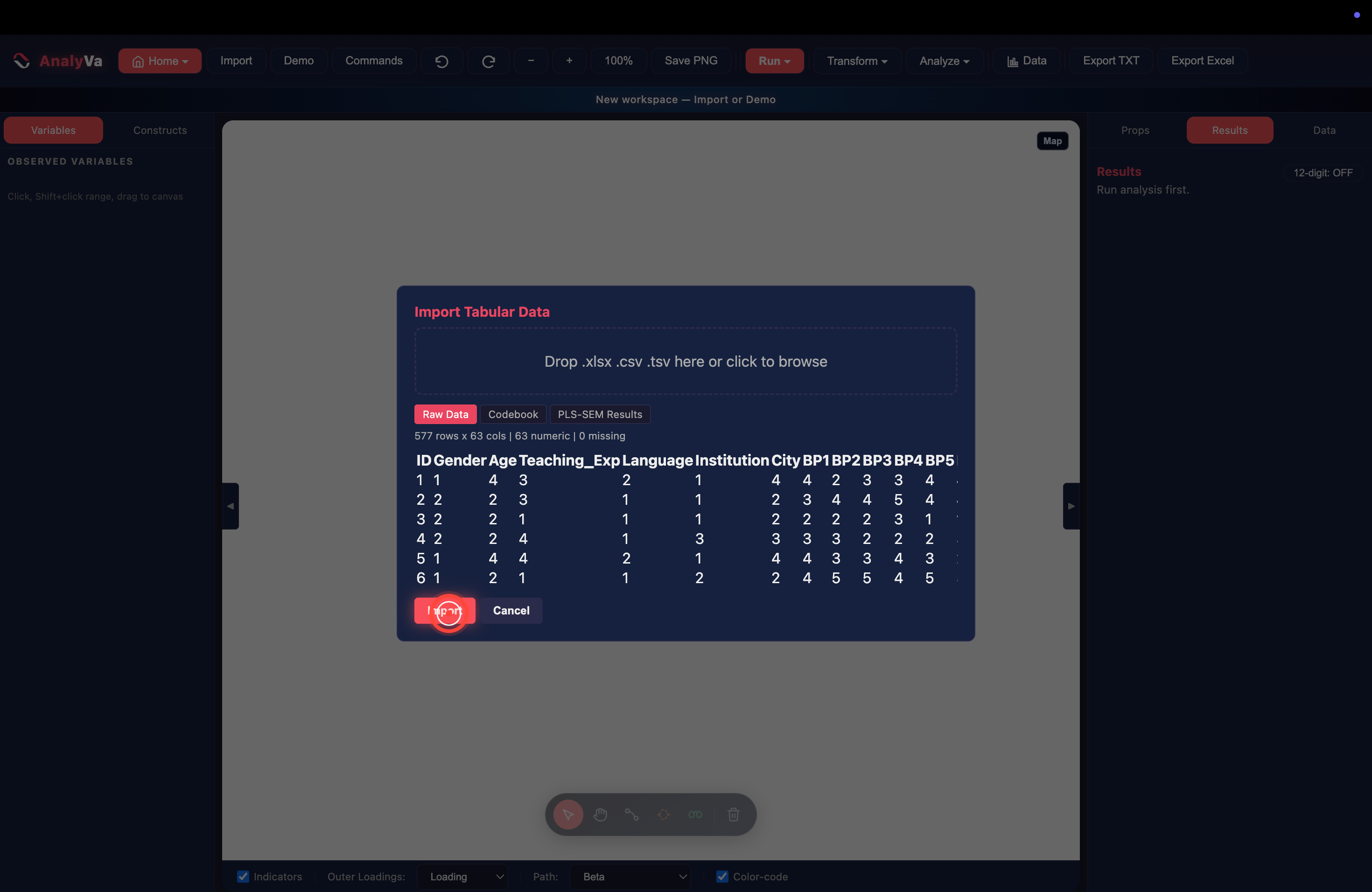
Step 2 — The import dialog opens. An overlay appears asking for a file. Accepts .xlsx, .csv, and .tsv.

Step 3 — Drop your file and preview. Drag your dataset onto the drop zone (or click to browse). AnalyVa parses it and shows the shape and the first rows for sanity-checking (here: 577 rows × 63 columns, all numeric, no missing values). Click Import when the preview looks right.

Step 4 — Open Analyze → Compare Means → Independent Samples t-test. Every variable in the dataset now appears in the left sidebar. Open the Analyze menu → Compare Means → Independent Samples t-test.

Step 5 — The t-test dialog opens. A dialog appears with sensible defaults filled in. AnalyVa auto-detects the grouping variable and its levels — here Gender has two groups, Group A = 1 (n = 234), Group B = 2 (n = 343).

Step 6 — Choose the test variable. Open the Test variable dropdown and pick the numeric variable you want to compare across the two groups. In this example: Teaching_Exp.

Step 7 — Click Run. The dialog now shows your chosen test variable, grouping variable, and both group sizes. Click the red Run button.

Step 8 — Read the results panel. The right pane switches to Results and shows every reporting component in one view:

• Group Descriptives — n, mean, SD, SE per group.
• Levene’s Test for Equality of Variances — F, p, and a plain-English “Equal Var?” verdict (here: Yes, p ≥ 0.05).
• t-test Results — both the equal-variance version (t = -0.582, df = 575, p = 0.560) and Welch’s (t = -0.580, df = 492.71, p = 0.562), with a checkmark on the one Levene recommends.
• Effect Size — Cohen’s d = -0.049, labelled Negligible.
• Box Plot Comparison — a side-by-side visualisation.

Notice how the interpretation lives right next to the p-value. You never have to hunt for the effect size, the assumption check, or the alternative test — everything a defensible report needs is in one scroll.

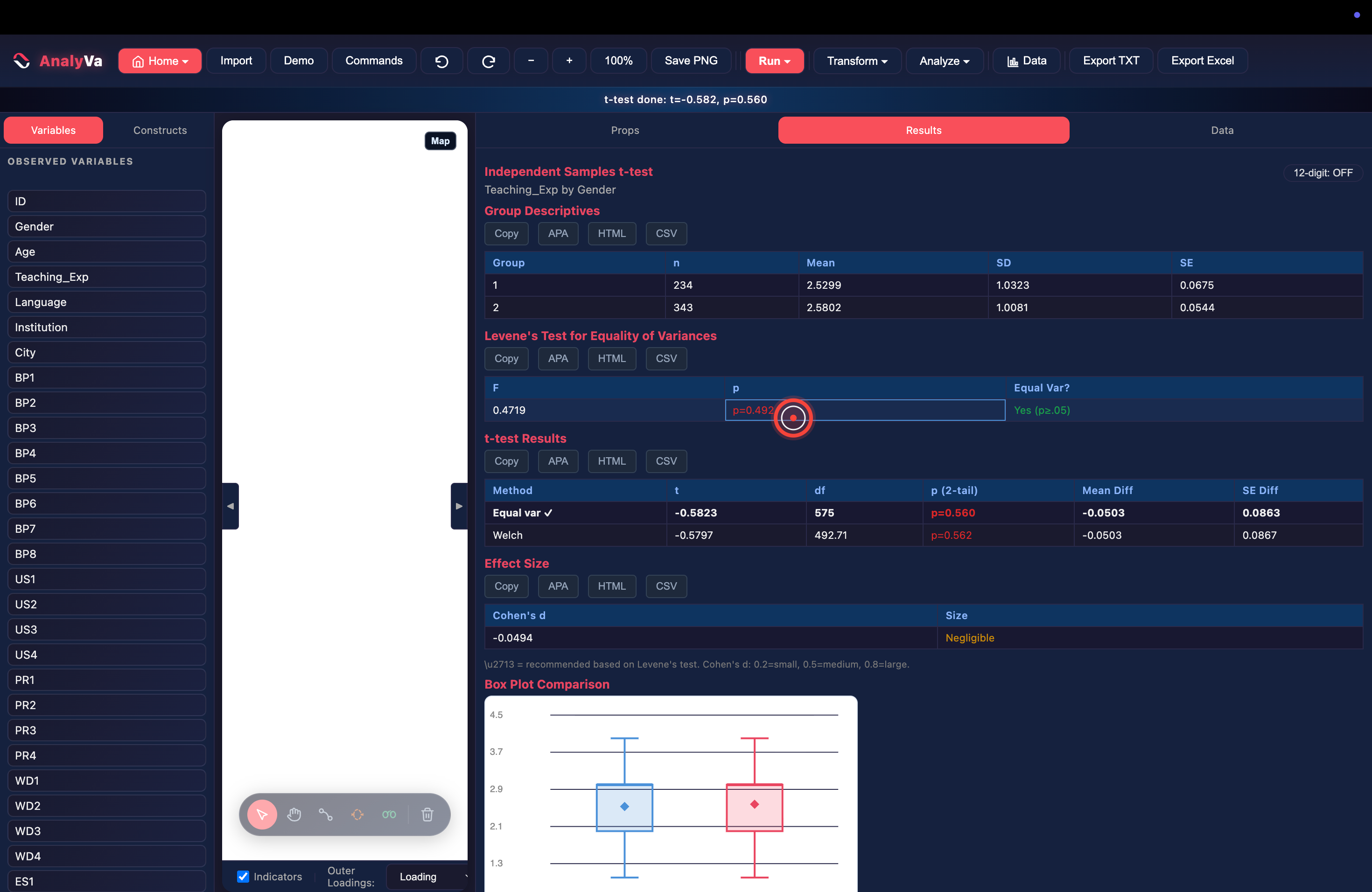
Every table has its own Copy, APA, HTML, and CSV button above it — so a properly formatted APA sentence (“t(575) = -0.58, p = .560, d = -0.05”) is one click away.

Further reading

• Wasserstein, R. L., & Lazar, N. A. (2016). The ASA’s statement on p-values: Context, process, and purpose. The American Statistician, 70(2), 129–133. DOI
• Amrhein, V., Greenland, S., & McShane, B. (2019). Scientists rise up against statistical significance. Nature, 567, 305–307.