The t-test is the workhorse of comparing means. But “the t-test” is really three related tests, and picking the wrong one is one of the most common mistakes in student and early-career research.

Here is the decision framework and the reporting standards.

The three t-tests

One-sample t-test. Compares one group’s mean to a known reference value. Example: are the students in this sample scoring above the national average of 100?

Independent-samples t-test. Compares the means of two different groups. Example: do men and women differ in exam scores?

Paired-samples t-test. Compares two measurements from the same subjects (or matched pairs). Example: did the students’ scores change from pre-test to post-test?

Using the wrong one inflates or deflates the Type I error rate. An independent test on paired data throws away statistical power; a paired test on independent data is simply invalid.

Decision tree

• Comparing one group to a fixed number? → one-sample.
• Comparing two independent groups? → independent.
• Comparing two measurements from the same subjects (or matched pairs)? → paired.
• Comparing three or more groups? → not a t-test. Use ANOVA.

Assumptions

All t-tests assume:

• the dependent variable is continuous (interval or ratio);
• observations are independent within each group;
• the dependent variable is approximately normally distributed within each group.

The independent-samples t-test additionally assumes equal variances between groups (homogeneity). When that is violated, use Welch’s t-test — most modern statistical software defaults to Welch’s for exactly this reason. It costs nothing when variances are equal and works correctly when they are not.

Effect size — report it, always

A p-value tells you whether a difference exists. Cohen’s d tells you how big it is.

• d = 0.20 → small
• d = 0.50 → medium
• d = 0.80 → large

A study with n = 1,000 might return p < .001 for d = 0.05 — statistically significant, practically meaningless. Always report d alongside its 95% confidence interval.

Three common mistakes

1. Running pairwise t-tests on three or more groups. Three groups A, B, C tested with three t-tests (A vs B, A vs C, B vs C), each at α = 0.05, gives a family-wise error rate of roughly 14%. Use ANOVA followed by a post-hoc test (Tukey’s HSD, Bonferroni) instead.

2. Ignoring Welch’s t-test. When group variances differ notably (Levene’s test p < 0.05), the classical Student’s t-test is biased. Welch’s has no such assumption. Modern journals expect Welch’s by default when variances are unequal.

3. One-tailed tests without prior justification. A one-tailed test doubles statistical power on one side, but requires you to have committed to a direction before looking at the data. Post-hoc one-tailed tests are a form of p-hacking. Report two-tailed by default unless you have a preregistered directional hypothesis.

What to report

For an independent-samples t-test, a defensible modern report:

“The intervention group scored significantly higher than the control group, t(48) = 3.21, p = .002, d = 0.91, 95% CI for d [0.34, 1.48].”

Components:

• t(df) = value — the statistic and its degrees of freedom.
• exact p — not just “< .05”.
• Cohen’s d plus its 95% CI.
• The mean difference plus its 95% CI where journal style allows.

Doing this in AnalyVa

The workflow is almost identical for all three t-test variants — the only real decision point is which one you pick from the menu in Step 4. This walkthrough uses an Independent Samples t-test as the worked example, and calls out at each step how the other two variants diverge.

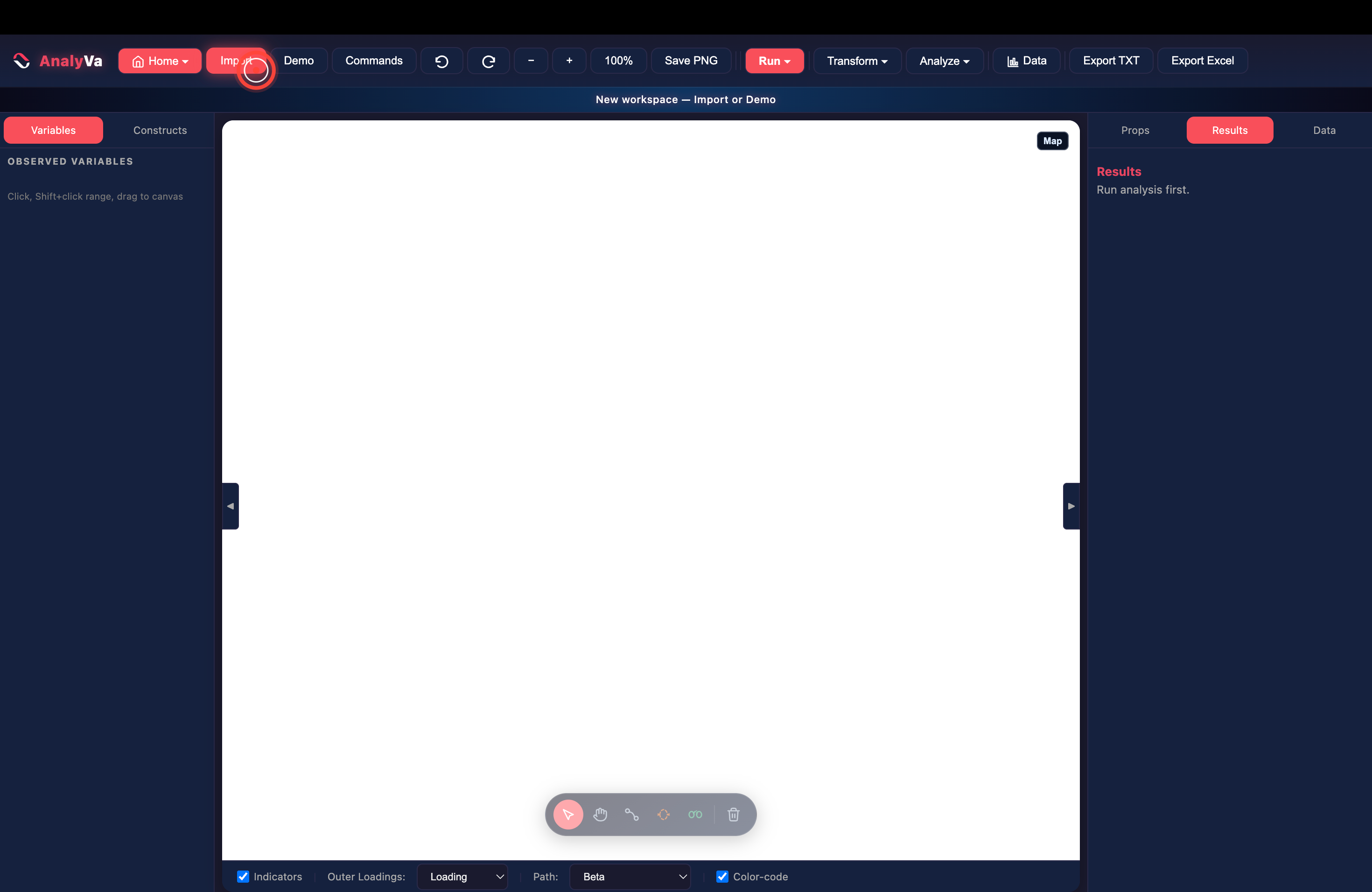
Step 1 — Click Import. Launch AnalyVa on an empty canvas. Click the Import button in the top toolbar.

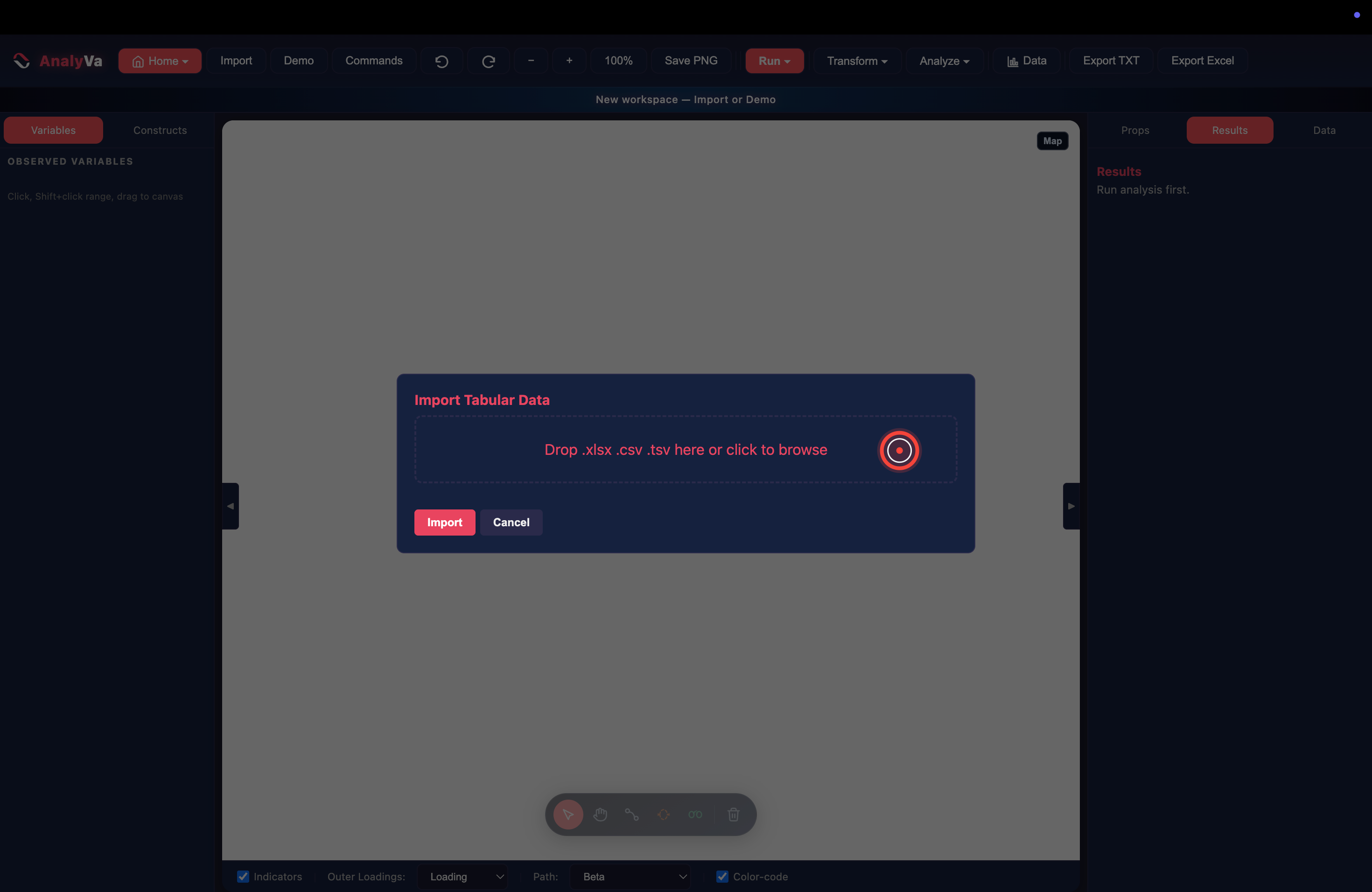
Step 2 — The import dialog opens. An overlay appears asking for a file (.xlsx, .csv, or .tsv).

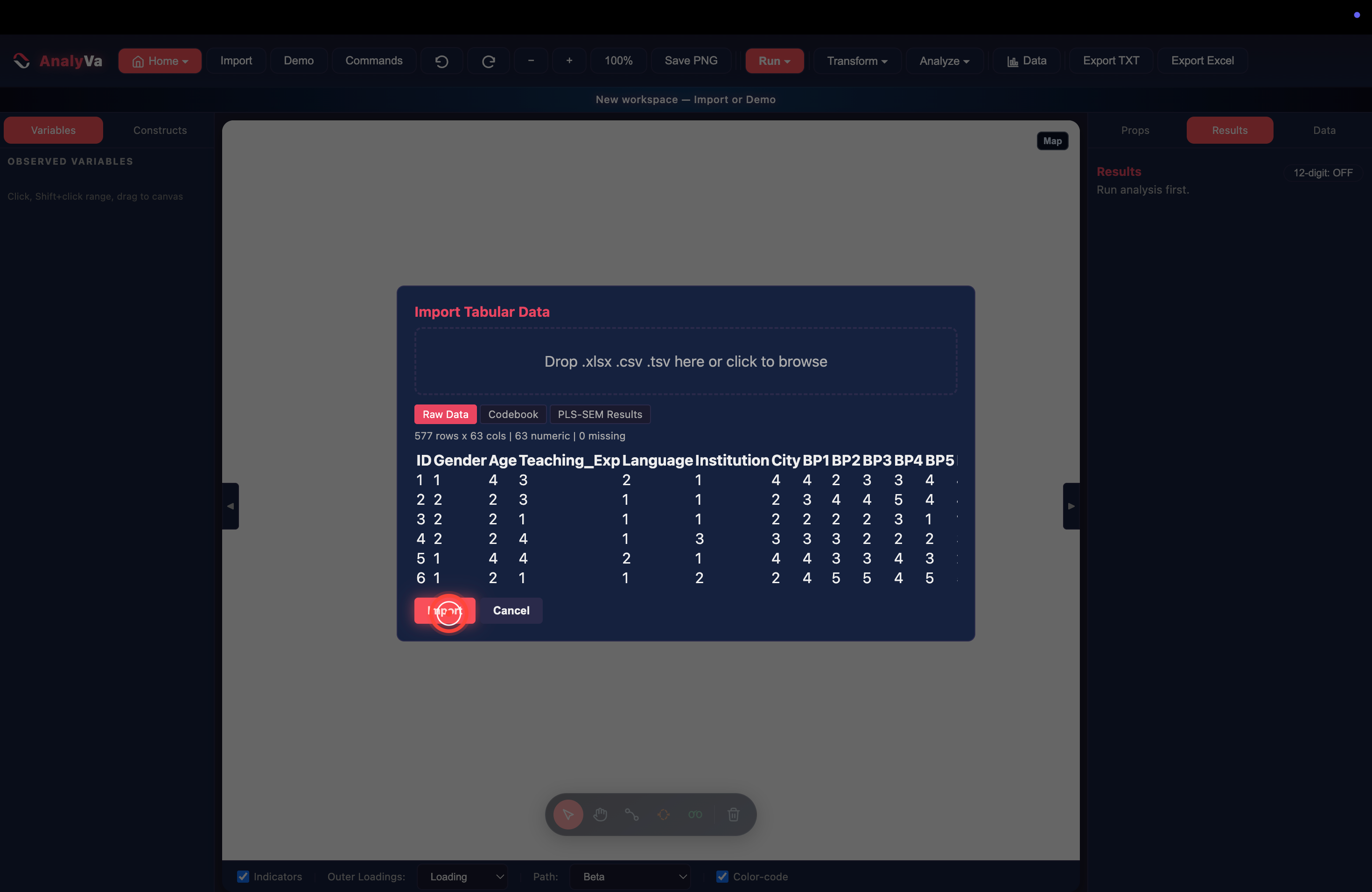
Step 3 — Load and preview. Drop your dataset. AnalyVa reports the shape and shows the first rows so you can confirm it parsed correctly. Click Import.

Your dataset needs to include:

• One-sample: the continuous variable of interest;
• Independent-samples: a continuous outcome + a grouping variable with exactly two levels;
• Paired-samples: two continuous variables measured on the same cases (pre + post, spouse-A + spouse-B, etc.).

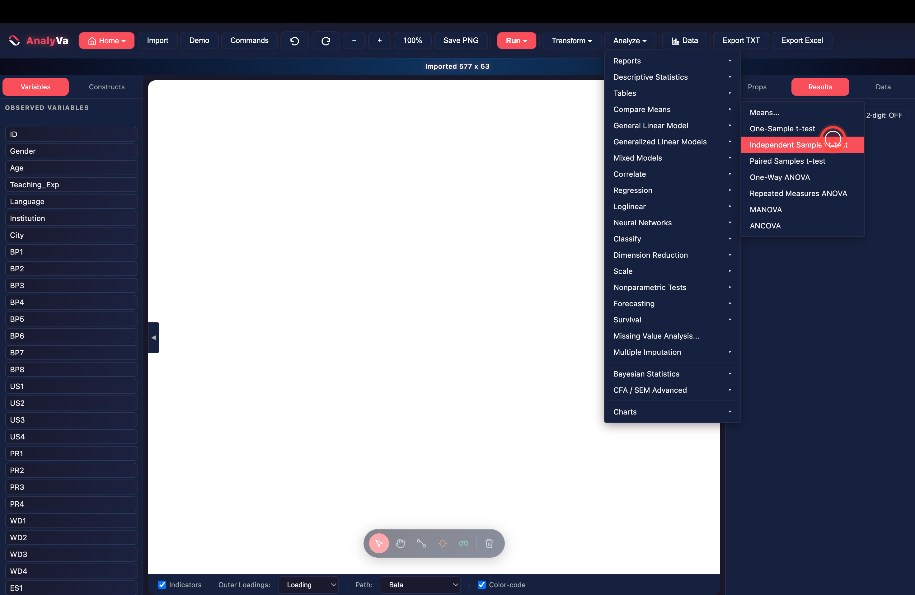
Step 4 — Pick the right t-test from Analyze → Compare Means. This is the only decision that changes. Open the Analyze menu → Compare Means. The submenu lists all three t-tests explicitly:

• One-Sample t-test — for comparing one group’s mean to a fixed reference value.
• Independent Samples t-test — for two different groups (this example).
• Paired Samples t-test — for two measurements from the same subjects.

If your design matches multiple items, re-read the decision tree earlier in this post — only one of them is appropriate for any given research question.

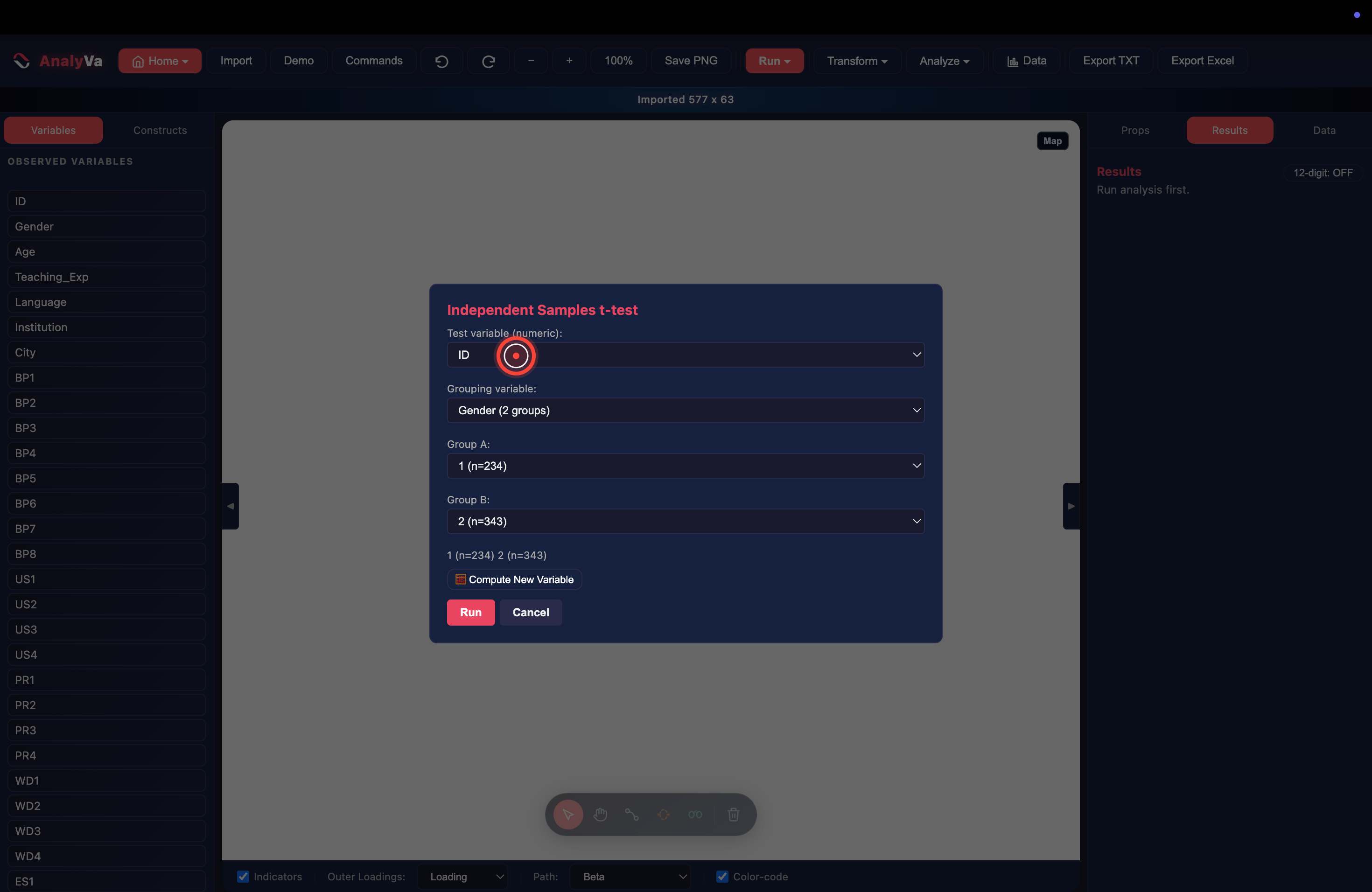
Step 5 — The test dialog opens with defaults. Pick Independent Samples t-test and AnalyVa opens a dialog with sensible defaults filled in. Here it auto-detected Gender as the grouping variable and mapped its two levels (Group A = 1, n = 234; Group B = 2, n = 343). The two group sample sizes appear as a one-line summary so you can catch obvious data errors immediately.

For the other two variants the dialog looks slightly different:

• The One-Sample dialog asks for a Test value — the reference number to compare the mean to (population norm, chance level, etc.).
• The Paired-Samples dialog asks for Variable 1 and Variable 2 — the two paired measurements on the same cases — instead of a test variable + a grouping variable.

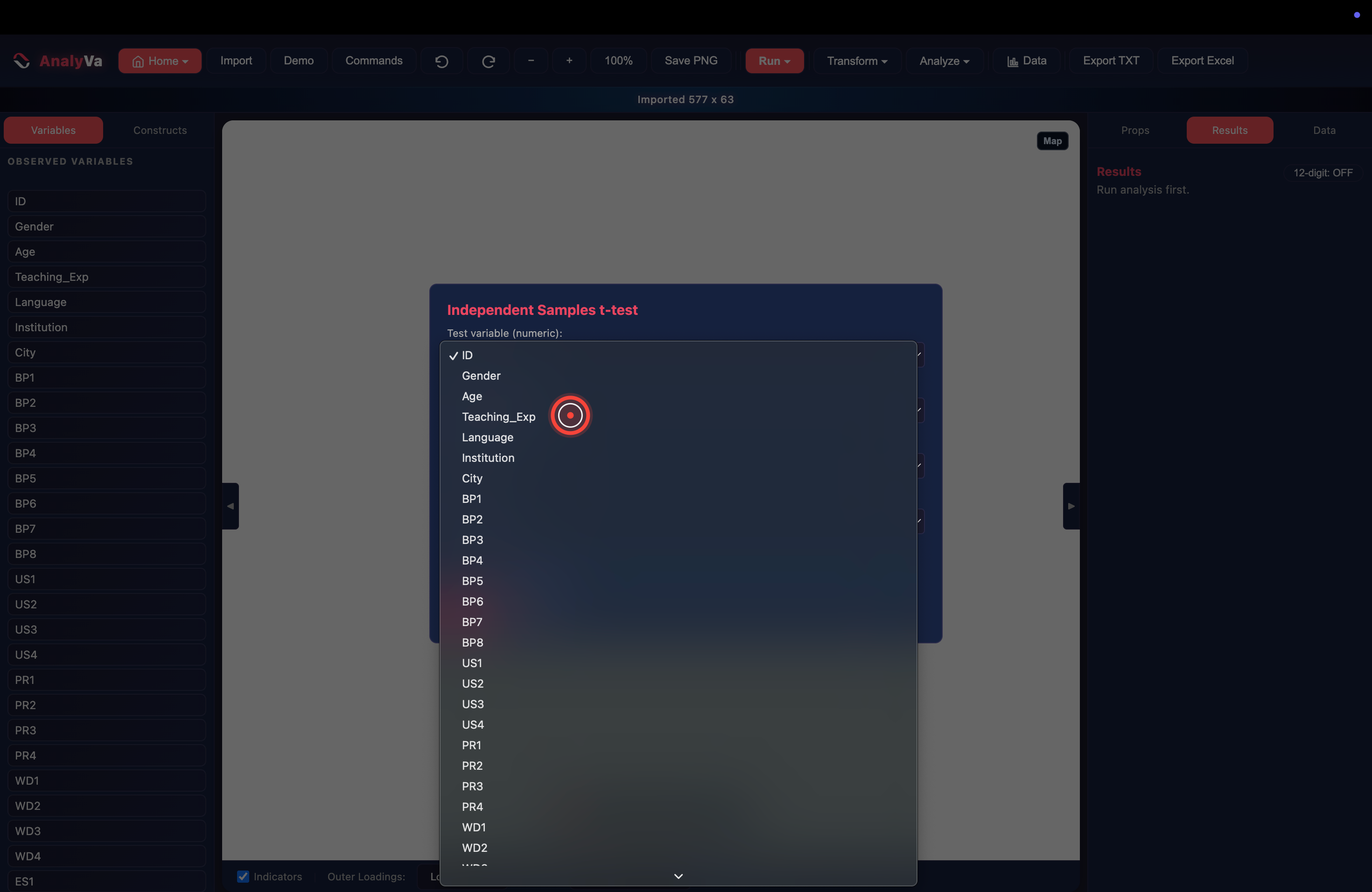
Step 6 — Choose the test variable. Open the Test variable dropdown and pick the numeric outcome you want to compare across the two groups. In this example: Teaching_Exp.

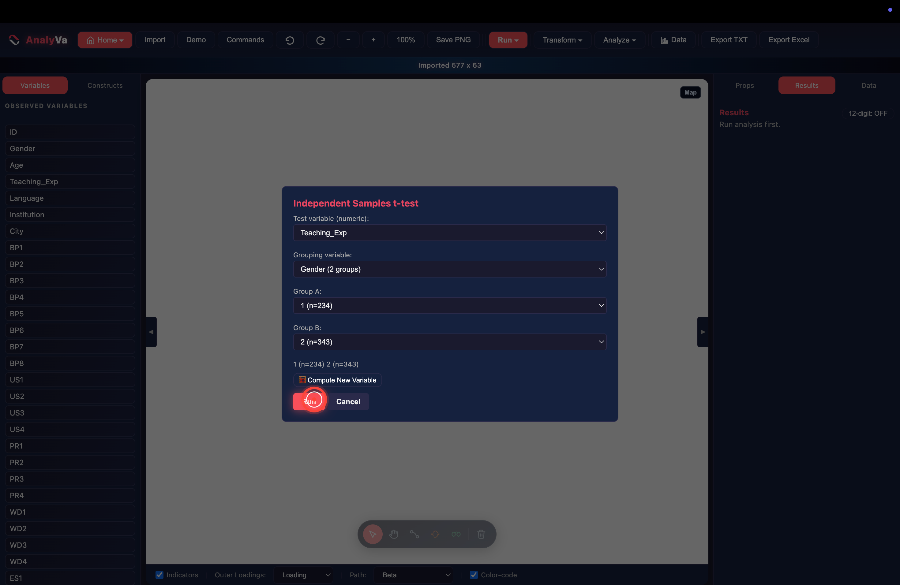
Step 7 — Click Run. The dialog now shows your chosen test variable, grouping variable, and both group sizes. Click the red Run button.

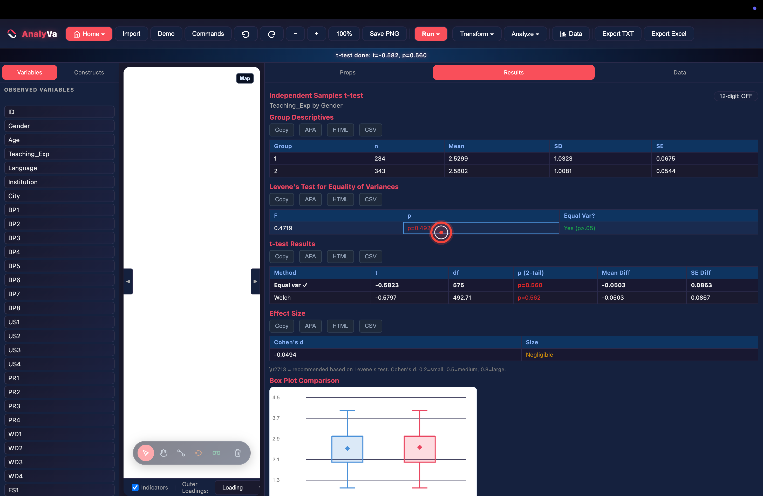
Step 8 — Read the results panel. The right pane switches to Results and shows everything a defensible t-test report needs, in one view:

• Group Descriptives — n, mean, SD, SE for each group.
• Levene’s Test for Equality of Variances — F, p, and a plain-English “Equal Var?” verdict. Here: Yes, p ≥ .05.
• t-test Results — both the classical Student’s version (t = -0.582, df = 575, p = .560) and Welch’s (t = -0.580, df = 492.71, p = .562), with a ✓ on whichever one Levene’s test recommends. You never have to remember which to report — AnalyVa flags it.
• Effect Size — Cohen’s d = -0.049, labelled Negligible. No hunting for the effect size in a separate output.
• Box Plot Comparison — a side-by-side visual so a reviewer can see the distributions at a glance.

For a paired t-test the same output appears with an extra Correlation between paired scores row and the mean of the differences instead of the mean difference between groups. For a one-sample test, Levene disappears (only one group) and the results compare the group mean to the reference value you specified.

Every table has Copy, APA, HTML, and CSV buttons. Click APA on the t-test Results table and it copies a ready-to-paste sentence like:

“t(575) = -0.58, p = .560, d = -0.05”

into your clipboard, ready to drop into the manuscript.

Further reading

• Lakens, D. (2013). Calculating and reporting effect sizes to facilitate cumulative science: A practical primer for t-tests and ANOVAs. Frontiers in Psychology, 4, 863.
• Delacre, M., Lakens, D., & Leys, C. (2017). Why psychologists should by default use Welch’s t-test instead of Student’s t-test. International Review of Social Psychology, 30(1), 92–101.