HTMT Above 0.85: What to Do When Discriminant Validity Fails

You ran PLS-SEM, opened the report, and one HTMT value is 0.87. The manuscript is due Friday. The reviewer you’re most worried about wrote their PhD on discriminant validity. What now?

This post gives you a concrete decision path — the same one used by methodologists like Henseler, Ringle, and Sarstedt (2015) and extended in later work. It applies whether you’re running the analysis in SmartPLS 4, in R with the SEMinR or cSEM packages, or in AnalyVa.

What HTMT actually measures

The Heterotrait-Monotrait ratio of correlations (HTMT) compares the average correlation of indicators across two constructs to the average correlation of indicators within each construct. When HTMT approaches 1.0, the two constructs are effectively measuring the same thing.

There isn’t one universally accepted cutoff. The three most commonly cited thresholds are:

HTMT < 0.85 — strict. Recommended when your constructs are conceptually distinct (e.g., trust vs. satisfaction).
HTMT < 0.90 — liberal. Acceptable when constructs are conceptually close (e.g., cognitive trust vs. affective trust).
HTMT confidence interval excludes 1.0 — the inferential test, based on bootstrap resampling. Preferred by many editors today.

If your value sits between 0.85 and 0.90, don’t panic yet — the inferential HTMT test is what most journals now expect you to report anyway.

The six things to try, in order

1. Check the bootstrapped HTMT confidence interval

Run 5,000 bootstrap subsamples with the percentile method and report the 97.5% upper bound. If the interval excludes 1.0, most reviewers will accept the constructs as empirically distinct even when the point estimate is above 0.85. This is the test that survives peer review.

2. Look at the offending indicator pair

HTMT is an average — it hides which specific pair is causing the problem. Pull the raw cross-loadings matrix and find the two indicators with the highest cross-construct correlation. That pair is usually where the theoretical overlap is real.

3. Consider whether the constructs are actually distinct

Sometimes HTMT is telling you the truth: the two constructs aren’t distinct in your data. This is the moment to step back from the statistics and ask a theoretical question. Are perceived usefulness and perceived value really separate for your sample, or did your respondents treat them as the same idea? If the constructs collapse conceptually, merge them and reestimate.

4. Drop the weakest cross-loading indicator

If the pair problem is driven by one indicator with a weak outer loading (< 0.70) and a strong cross-loading, drop it. Document the decision in the methods section. Never drop indicators purely to “fix” HTMT — you need a defensible measurement reason.

5. Reconsider the reflective/formative specification

If one of the constructs is actually formative (its indicators cause the latent variable rather than reflect it), HTMT doesn’t apply in the first place. Formative constructs are assessed with VIF and indicator weights, not with HTMT or AVE. Misspecification is a common hidden cause of “failing” discriminant validity.

6. If all else fails, report and defend

If the theory supports two distinct constructs, the bootstrapped HTMT interval excludes 1.0, and dropping indicators would harm construct coverage, report the HTMT value honestly and defend it in the Discussion. Editors generally accept a defended 0.87 more readily than a suspiciously clean 0.84 that clearly came from indicator surgery.

How this looks in SmartPLS 4

SmartPLS 4 reports the HTMT point estimate in the standard PLS algorithm output, and the bootstrapped confidence intervals under the “Discriminant Validity” tab after you run the bootstrap procedure. To identify the offending indicator pair, open the “Cross Loadings” report.

Doing this in AnalyVa

The full workflow, from a fresh canvas to an HTMT verdict on every construct pair in the model.

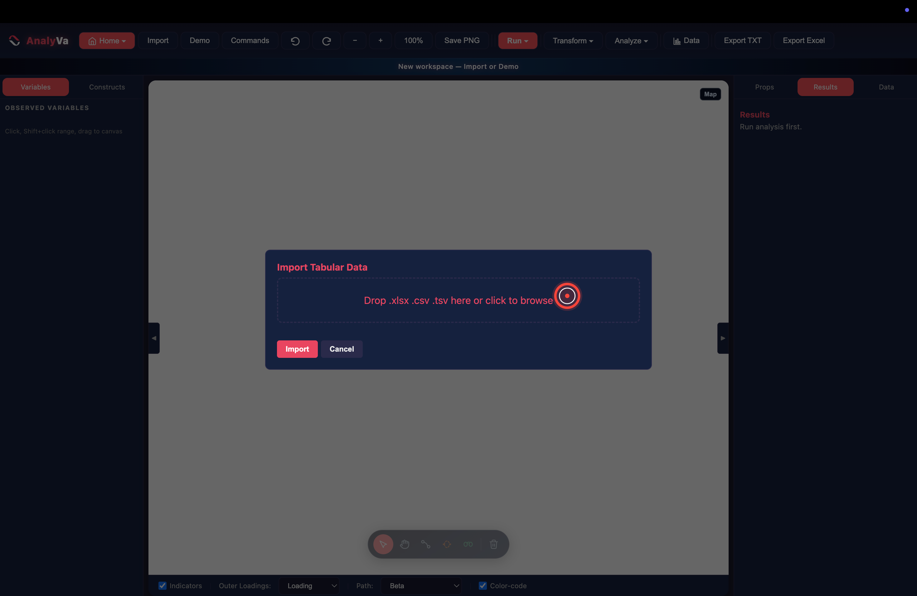
Step 1 — Click Import. Launch AnalyVa on an empty canvas. Click the Import button in the top toolbar.

Step 2 — The import dialog opens. An overlay appears asking for a file (.xlsx, .csv, or .tsv).

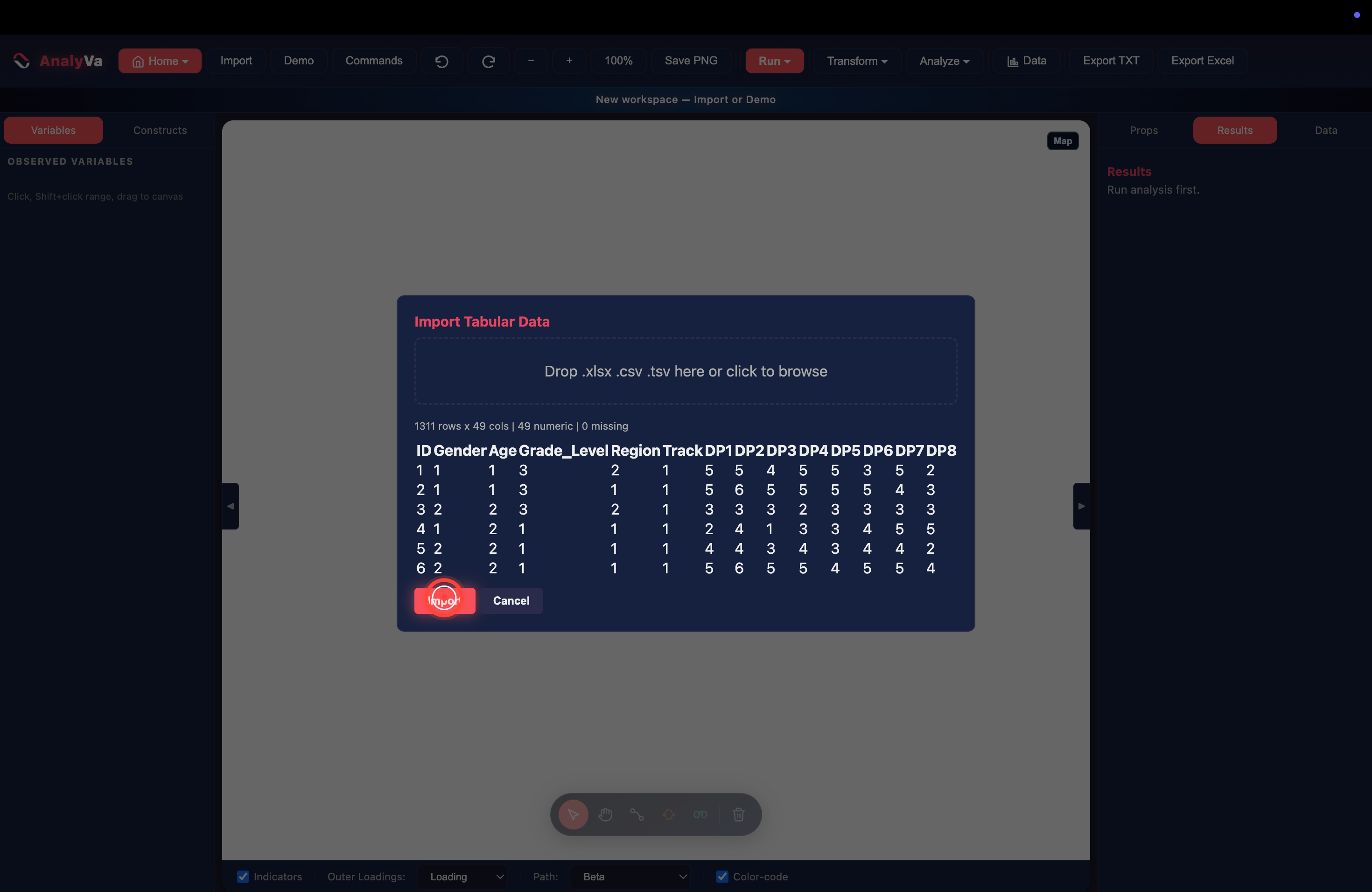
The Import Tabular Data dialog waiting for a file

Step 3 — Load the file and preview it. Drop your dataset. AnalyVa parses it and reports the shape (here: 1,311 rows × 49 columns, all numeric, no missing). The first six rows appear so you can sanity-check. Click Import.

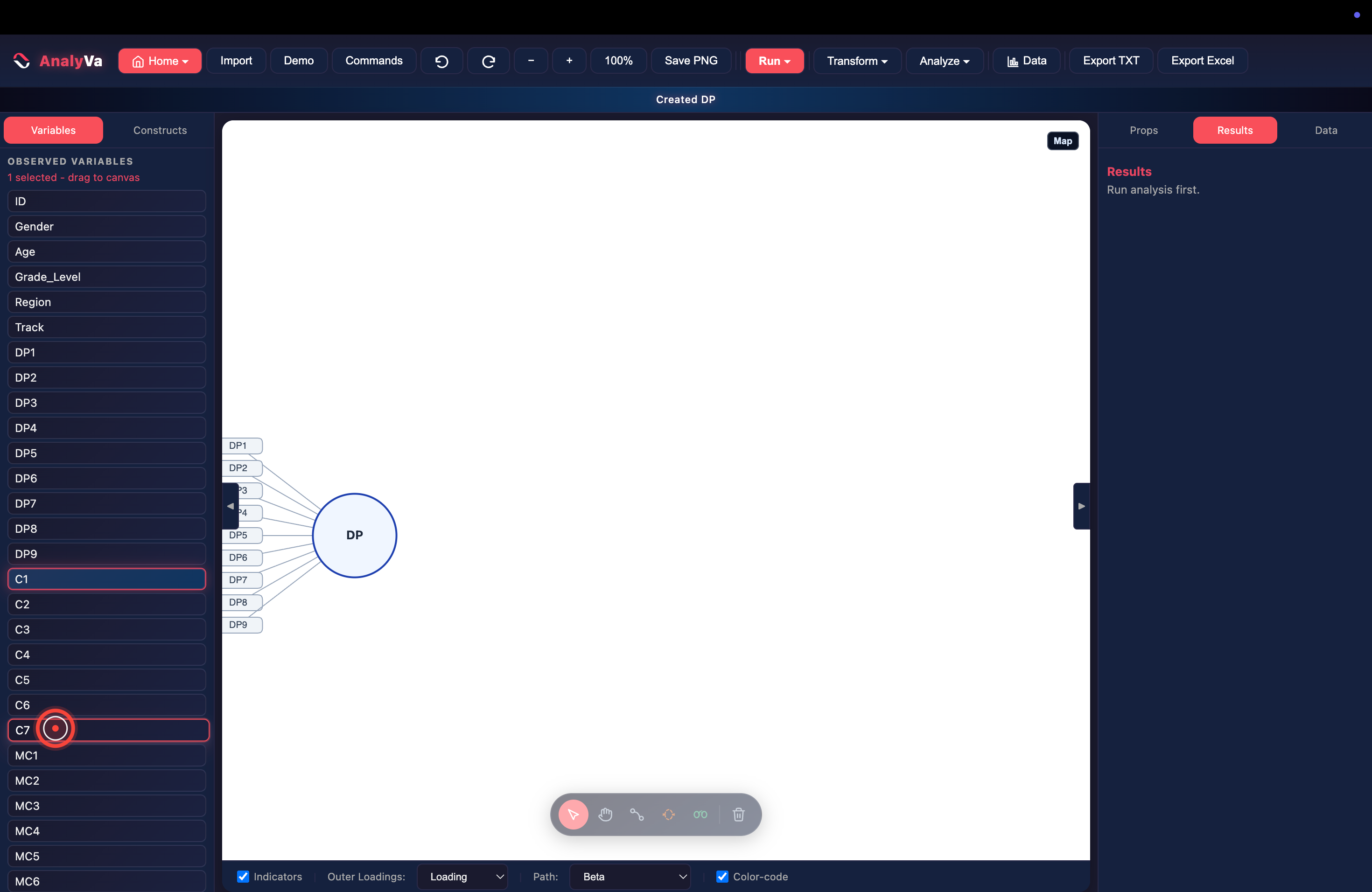
The Import dialog showing the file preview and the Import button

Step 4 — Build the first construct. Every variable now appears in the sidebar. To create a construct, click its first indicator in the sidebar (here, C1).

The sidebar with C1 selected

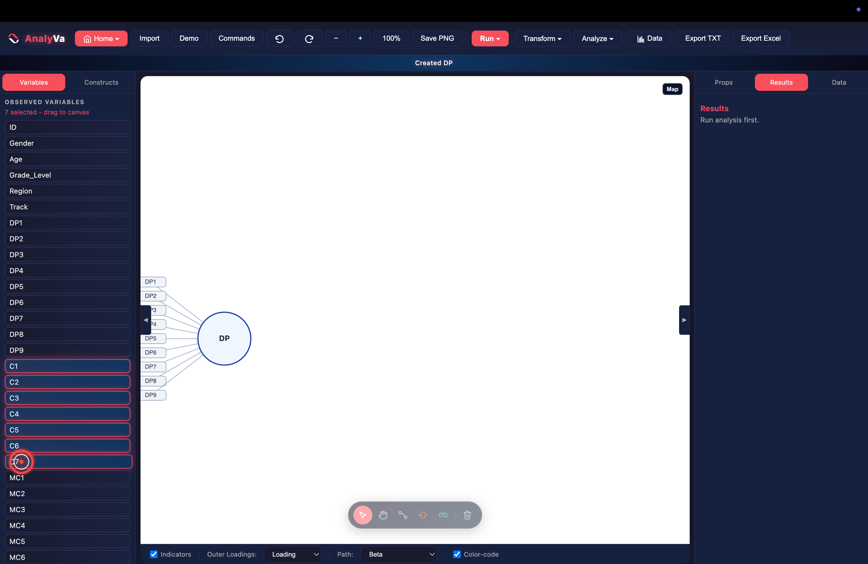
Step 5 — Shift-click the last indicator to select the range. Shift-click C7 (or Ctrl/Cmd-click individual items). The sidebar highlights the whole range in red. Then drag the selection onto the canvas — AnalyVa creates a construct named after the item prefix (here: C) with all 7 indicators attached.

All 7 C items highlighted in the sidebar

Step 6 — Repeat for the second construct. The canvas now shows two constructs (C and DP — DP was created the same way earlier). To add the third, click the first indicator of the new construct in the sidebar (here: MC1).

MC1 selected in the sidebar

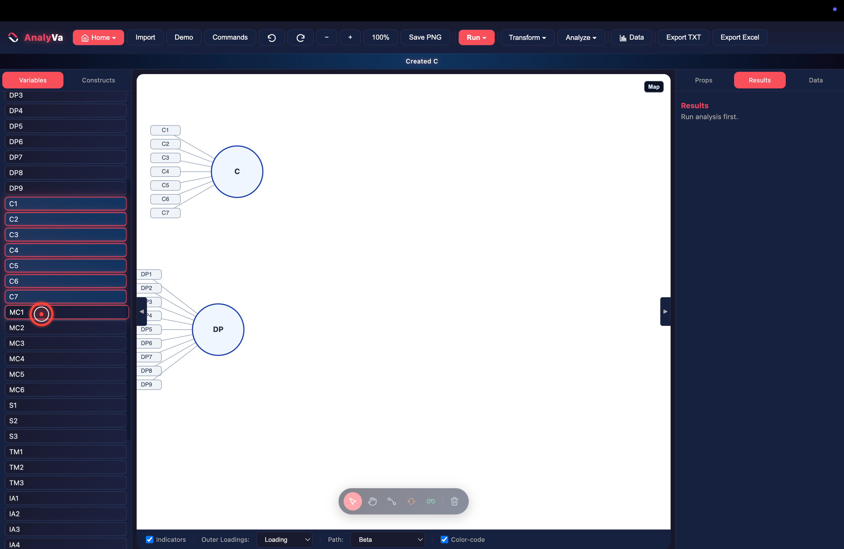
Step 7 — Shift-click through the range. Shift-click MC6 to select all six MC items.

MC1–MC5 highlighted, cursor on MC6

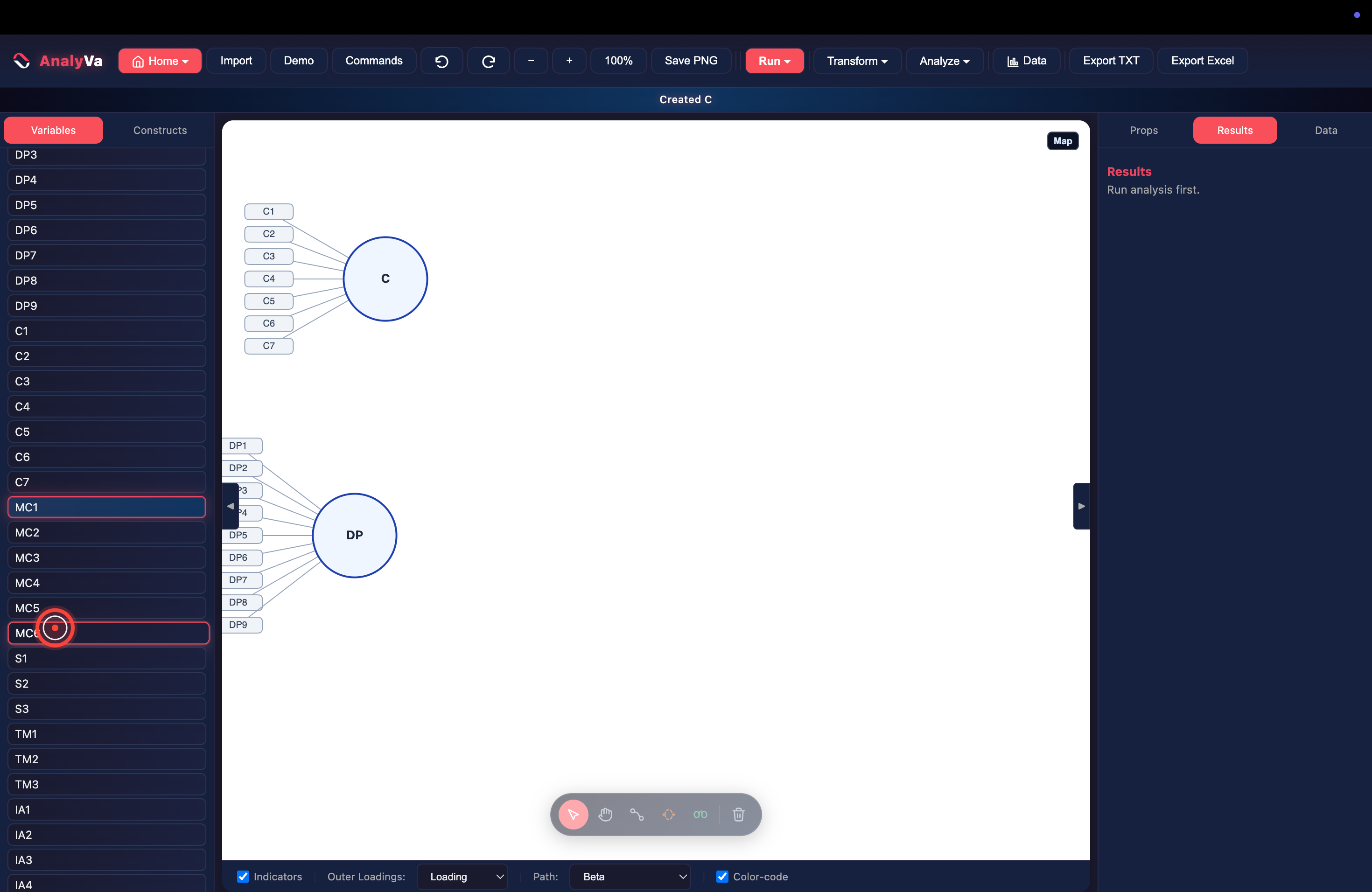
Step 8 — All six items selected. The MC block is now fully highlighted in the sidebar.

All 6 MC items highlighted

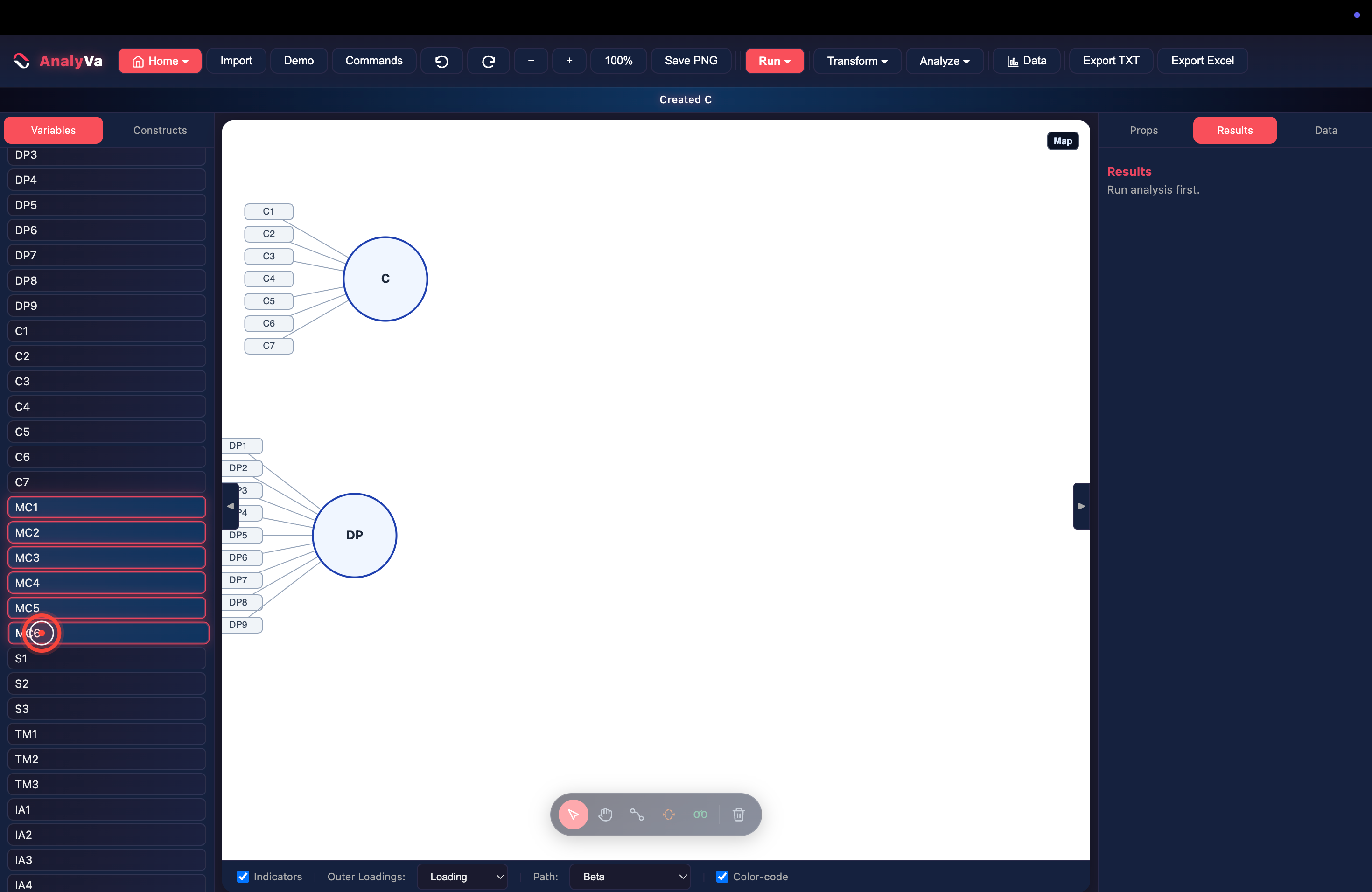
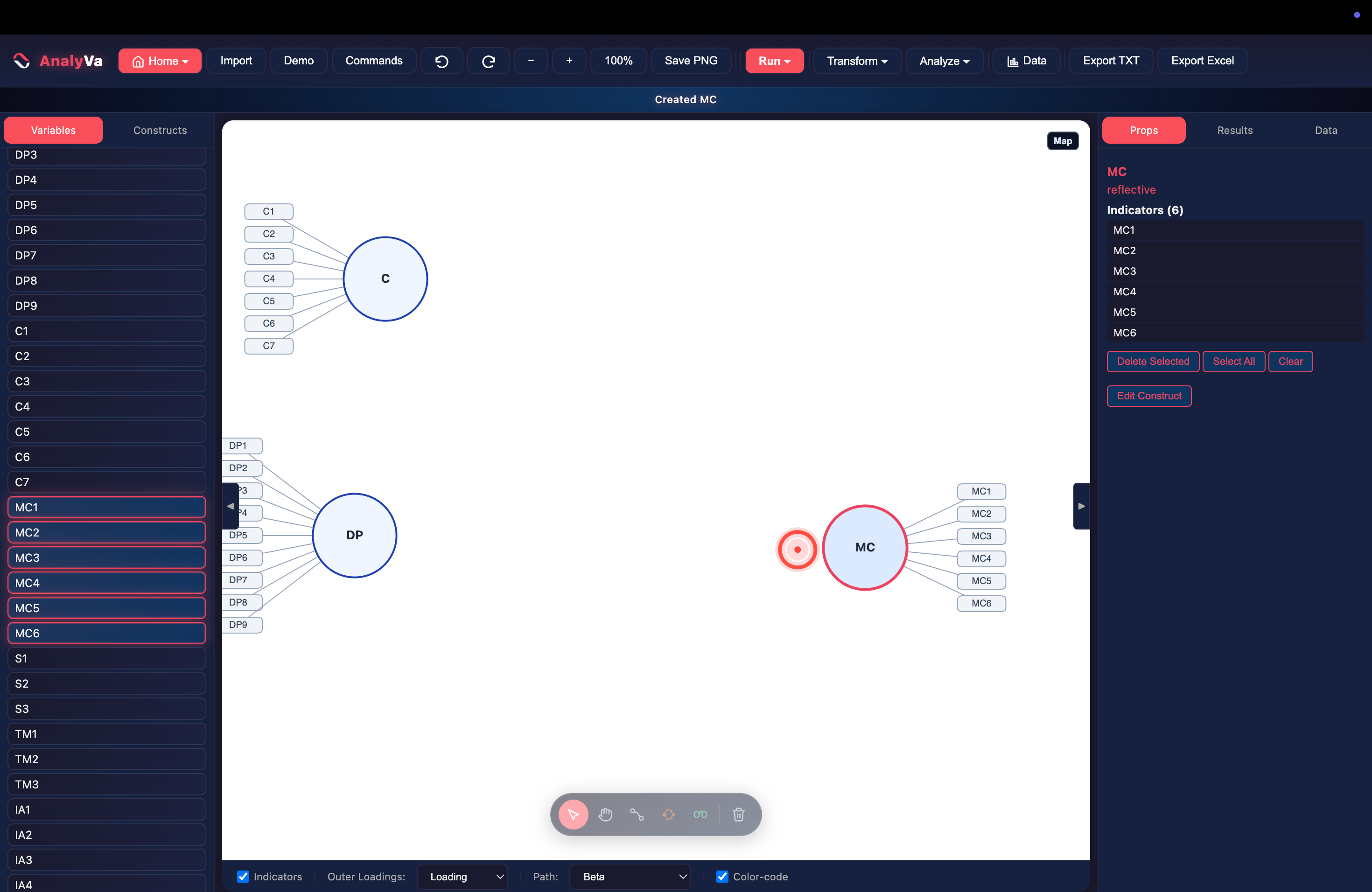
Step 9 — Drop the MC construct onto the canvas. Drag the highlighted MC items onto the canvas. AnalyVa creates the MC construct with all 6 indicators. Click the new construct — the right pane switches to Props and shows its type (reflective) and indicator list.

The MC construct on the canvas with its Props panel visible

Step 10 — Switch to the Path tool. At the bottom of the canvas is a small floating toolbar. The second button from the left is the Path (P) tool — click it (or press P).

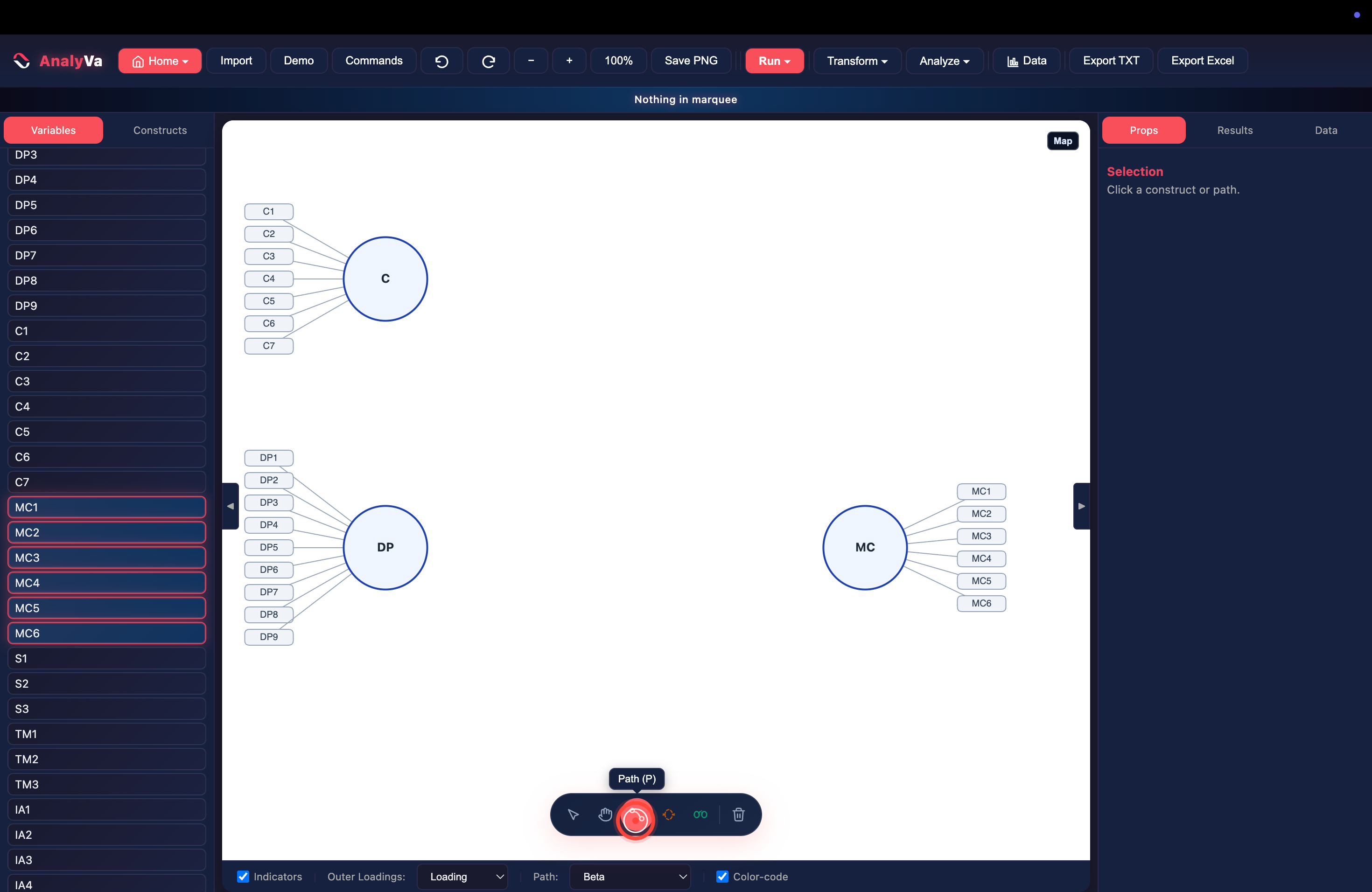
The Path tool in the floating toolbar

Step 11 — Start drawing a path. With the Path tool active, click the source construct. The cursor is now attached to that construct.

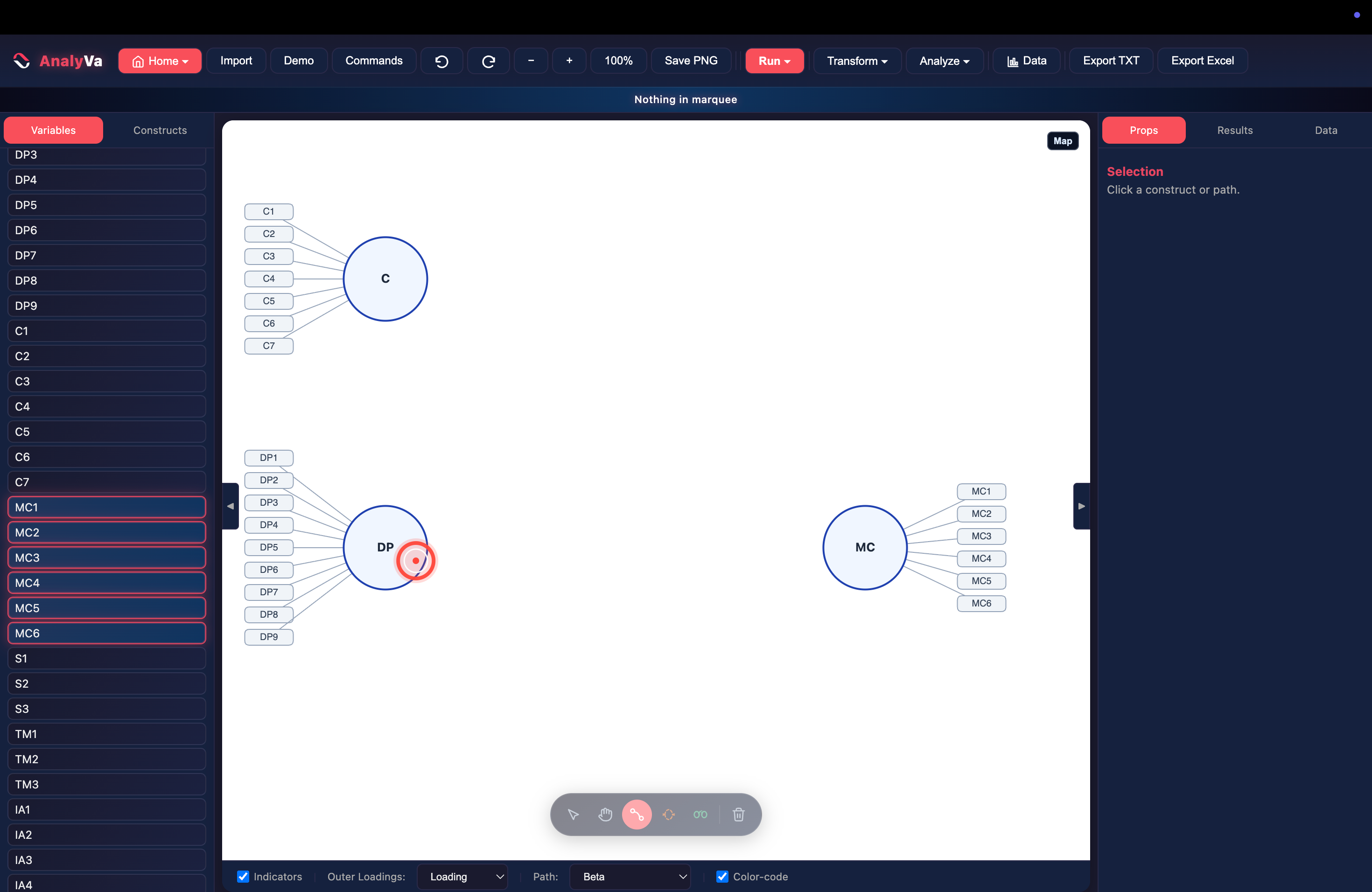
Path tool active, cursor on the DP construct

Step 12 — Draw H1: DP → MC. Click the target construct to complete the path. AnalyVa auto-labels it H1 and displays the hypothesis in the header bar (“H1: Path: DP -> MC”).

The first path H1 drawn from DP to MC

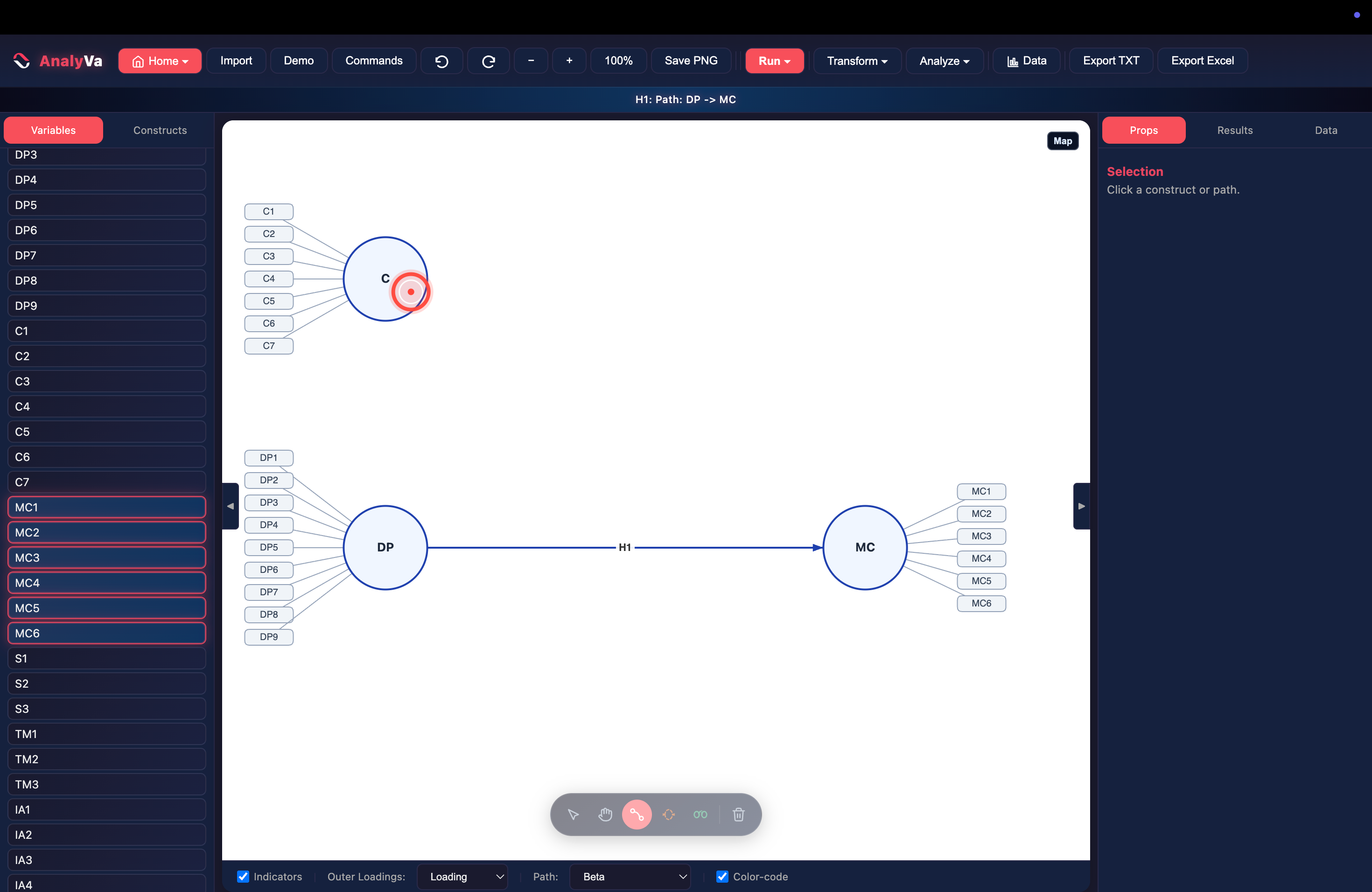
Step 13 — Draw H2: C → MC. Click C, then click MC. Path H2 is drawn.

H1 and H2 paths on the canvas

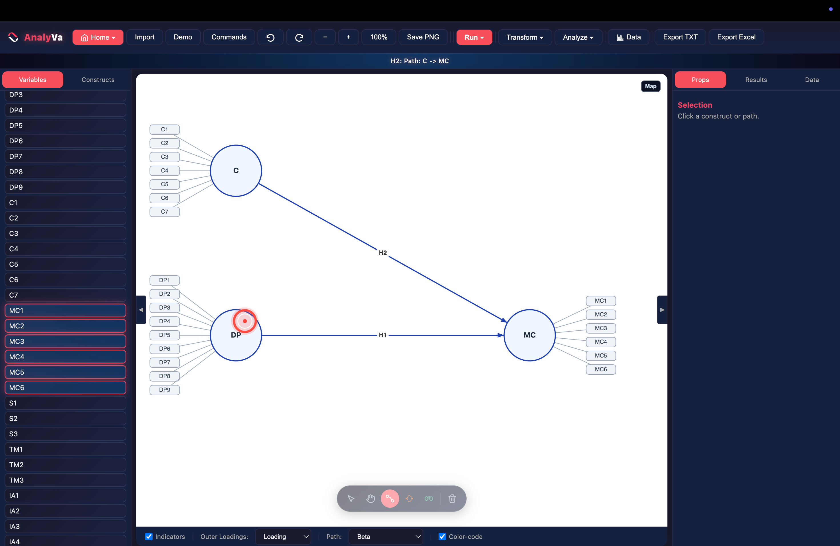
Step 14 — Draw H3: DP → C. Click DP, then click C. All three hypothesis paths are now drawn. The header confirms “H3: Path: DP -> C”.

All three paths drawn — H1, H2, H3

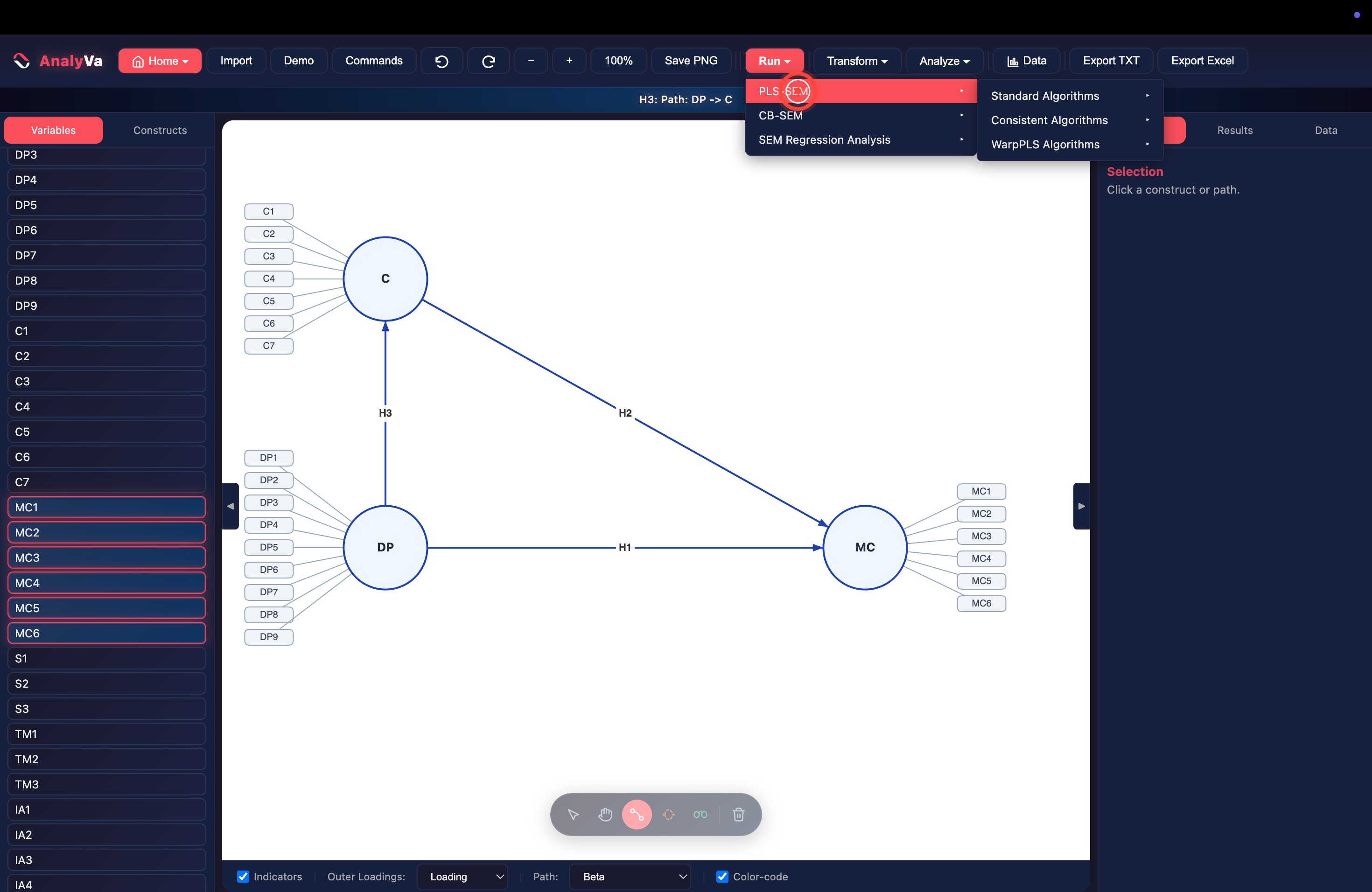
Step 15 — Open Run → PLS-SEM → Standard Algorithms → PLS-SEM algorithm. The model is ready to estimate. Open the Run menu → PLS-SEM → Standard Algorithms → PLS-SEM algorithm.

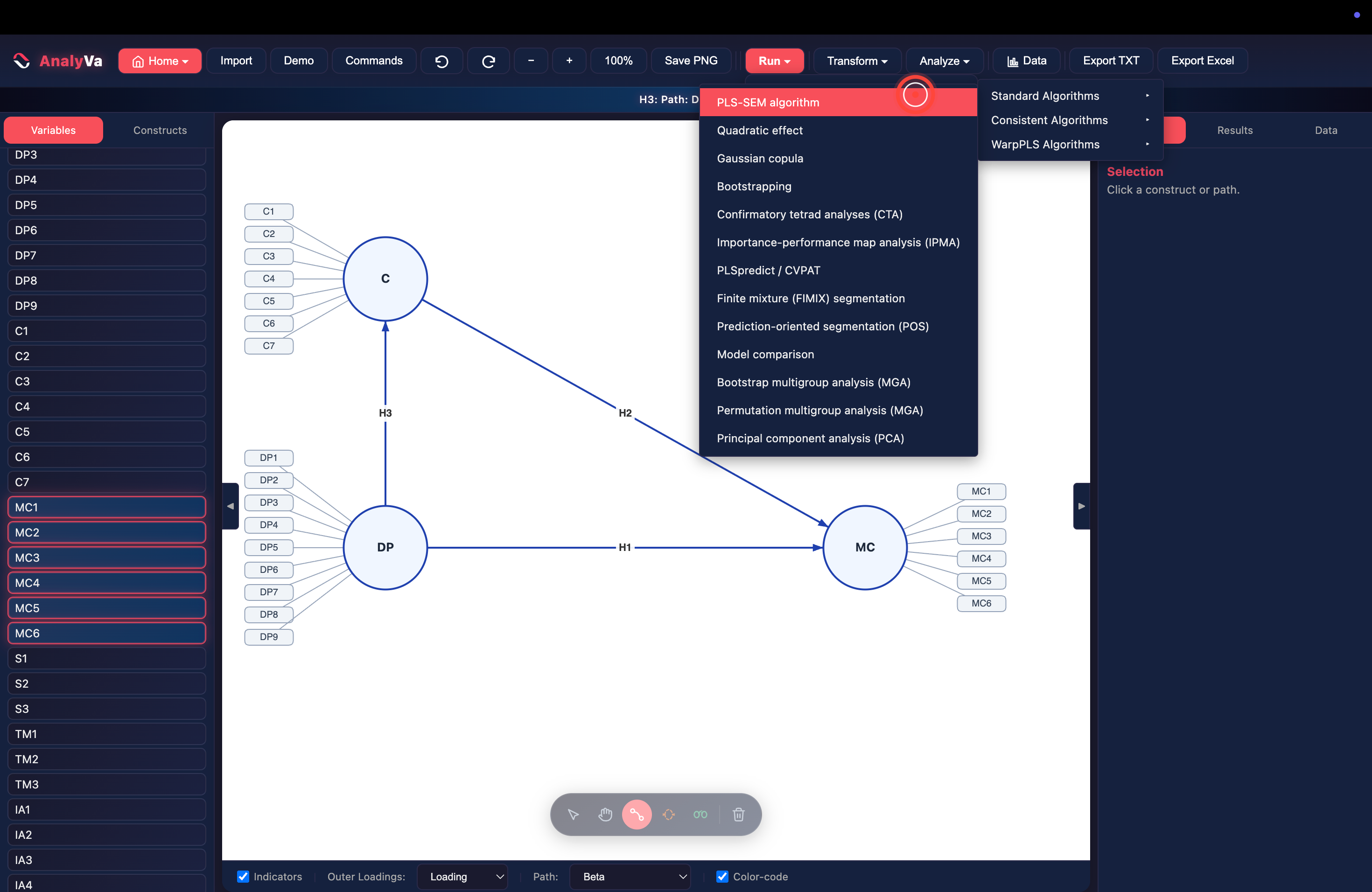
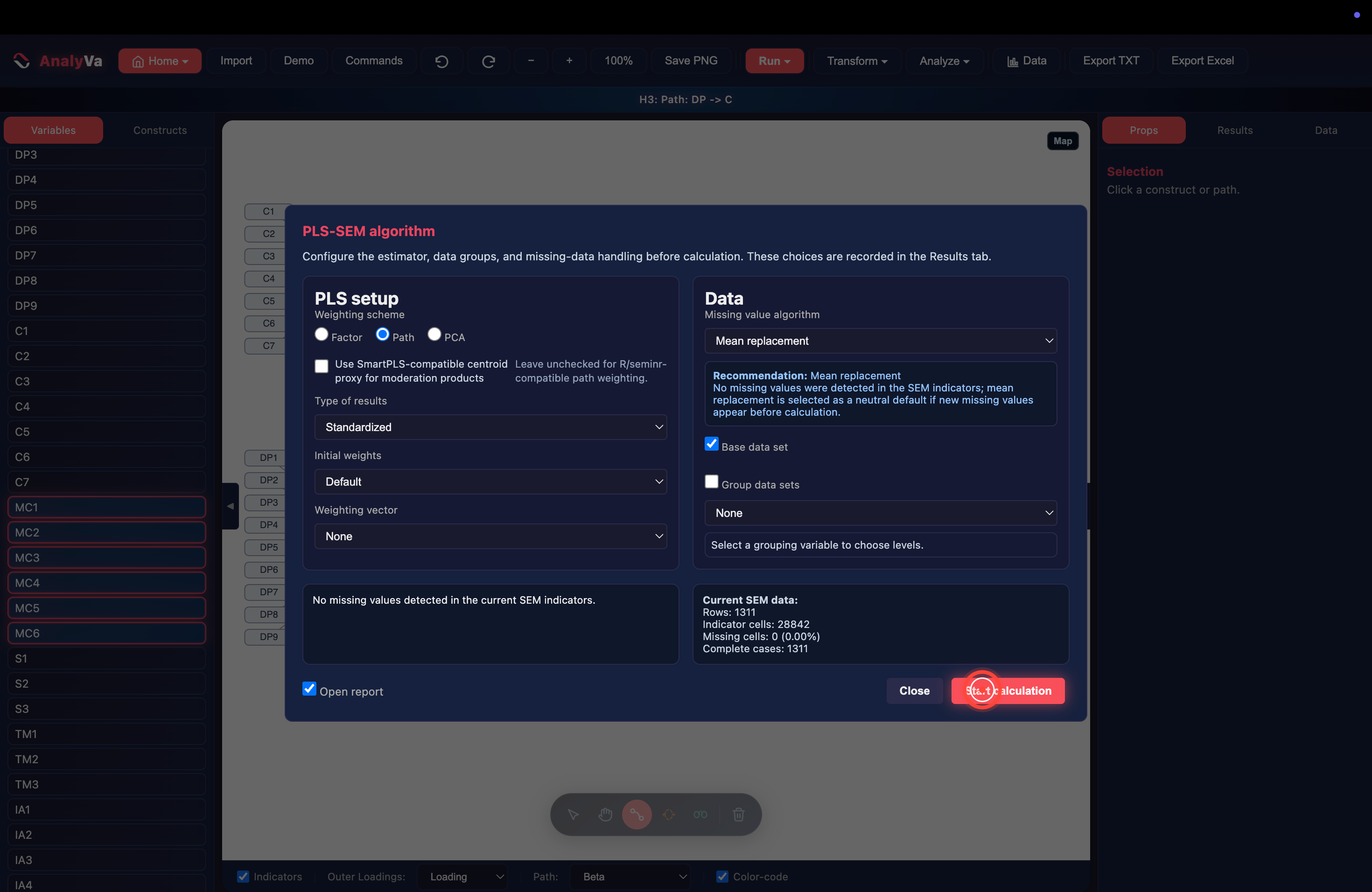
Step 16 — Configure and Start calculation. A configuration dialog opens: weighting scheme (Factor / Path / PCA), initial weights, missing-value handling. The defaults are the Hair et al. recommendations (Path weighting, mean replacement) and AnalyVa also reports the current data profile — 1,311 rows, 28,842 indicator cells, 0 missing. Leave the defaults and click Start calculation.

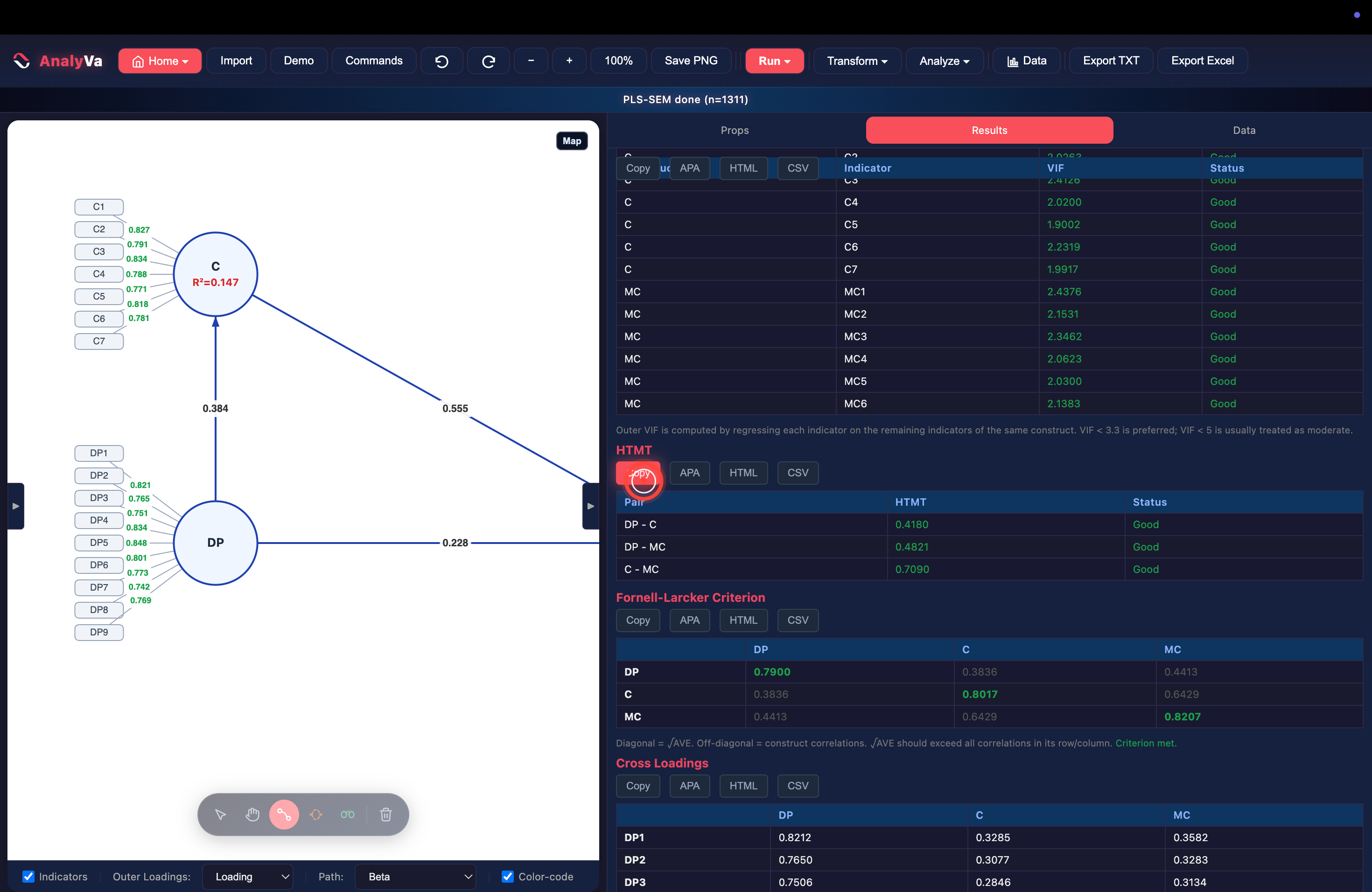
The PLS-SEM algorithm configuration dialog with Start calculation highlighted

Step 17 — Read the HTMT table. The right pane switches to Results and streams every report the Hair et al. checklist requires. The HTMT table sits high on the page with the verdict already labelled:

DP – C: 0.4180 → Good
DP – MC: 0.4821 → Good
C – MC: 0.7090 → Good

All three pairs are safely below 0.85. Outer VIF, Fornell-Larcker, cross-loadings, and the path diagram with computed loadings (0.827, 0.791, …) and path coefficients (0.384, 0.555, 0.228) are all generated in the same run — nothing to re-execute.

If any HTMT pair here had exceeded 0.85, the workflow to fix it starts right back at the top of this post: check the bootstrap CI, find the offending indicator pair in the cross-loadings table below, and decide.

The Results panel showing the HTMT table with all three construct pairs marked Good

Validation

AnalyVa’s HTMT calculations were benchmarked against SmartPLS 4 on the corporate reputation dataset (n = 344) as part of the second validation study. Point estimates and bootstrapped confidence intervals reproduce SmartPLS output to the reported precision. See the study on Zenodo at doi.org/10.5281/zenodo.21536948.